install.packages("rio")
install.packages("tidyverse")
install.packages("bupaverse")
install.packages("processanimateR")14 The Why, the How and the When of Educational Process Mining in R
Abstract
This chapter presents the topic of process mining applied to learning analytics data. The chapter begins by introducing the fundamental concepts of the method, with a focus on event log construction and visual representation using directly-follows graphs. A review of the existing literature on educational process mining is also presented to introduce the reader to the state of the art of the field. The chapter follows with a guided tutorial in R on how to apply process mining to trace log data extracted from an online learning management system. The tutorial uses the bupaverse framework for data handling and visualization. We finish the chapter with a reflection on the method and its reliability and applicability.
1 Introduction
Nowadays, almost all learning platforms generate vast amounts of data that include every interaction a student has with the learning environment. Such large amounts of data offer a unique opportunity to analyze and understand the dynamics of the learning process. In the previous chapters of the book, we covered several methods for analyzing the temporal aspects of learning, such as sequence analysis [1, 2], Markovian modeling [3] or temporal network analysis [4]. In this chapter, we present an analytical method that is specifically oriented at analyzing time-stamped event log data: process mining. Process mining is a technique that allows us to discover, visualize, and analyze the underlying process from time-stamped event logs. Through process mining, we may uncover hidden patterns, bottlenecks, and inefficiencies in students’ learning journeys. By tracking students’ actions step-by-step, we can identify which resources are most effective, which topics are more challenging, and even predict possible problems before they may occur.
Process mining emerged as a business tool that allows organizations to analyze and improve their operational processes. The field has rapidly expanded with several modelling methods, algorithms, tools and visualization techniques. Further, the method has been met with enthusiasm from several researchers leading to a rapid uptake by other disciplines such as health care management and education. As the field currently stands, it is a blend of process management and data science with less emphasis on statistical methods. The field has found its place in educational research with the recent surge of trace log data generated by students’ activities and the interest that learning analytics and educational data mining have kindled.
This tutorial chapter will introduce the reader to the fundamental concepts of process mining technique and its applications in learning analytics and education research at large. We will first describe the method, the main terminology, and the common steps of analysis. Then, we will provide a review of related literature to gain an understanding of how this method has been applied in learning analytics research. We then provide a step-by-step tutorial on process mining using the R programming language and the bupaverse framework. In this tutorial, we analyze a case study of students’ online activities in an online learning management system using the main features of process mining.
2 Basic steps in process mining
The goal of process mining is to extract process models from event data. The resulting models can then be used to portray students’ pathways in learning, identify common transitions, and find issues of their approach. In doing so, process mining promises to find deviations from the norm, suggest corrective actions, and optimize processes as an ultimate goal [5]. Process mining starts by the extraction of event data. In the case of educational process mining, event data often reflects students’ activities in learning management systems (LMSs), or in other types of digital tools that record time-stamped events of students’ interactions with the digital tools, such as automated assessment tools or online learning games. The said data is used to construct what is known as an event log. An event log has three necessary parts:
Case identifier: A case represents the subject of the process. For example, if we are analyzing students’ enrollment process, each student would represent a different case. If we are analyzing students’ online activities in the LMS, we can also consider each student as a separate case; alternatively, if we want a greater level of granularity, each student’s learning session can be then considered a separate case. All event logs need to have a case identifier that unequivocally identifies each case and that allows to group together all the events that belong to the same case.
Activity identifier: Activities represent each action or event in the event data. Continuing with the previous examples, an activity would represent each step in the enrollment process (e.g, application, revision, acceptance, payment etc.), or each action in the LMS (e.g., watch video, read instructions, or check calendar).
Timestamp: The timestamp is a record of the moment each event has taken place. It allows to establish the order of the events. In the case of online activity data, for instance, the timestamp would be the instant in which a student clicks on a learning resource. In some occasions, activities are not instantaneous, but rather have a beginning and an end. For example, if we are analyzing student’s video watching, we might have an event record when they start watching and when they finish. If we want to treat these events as parts of the same activity, we need to provide additional information when constructing an event log. As such, we need to specify an activity instance identifier, which would allow us to unequivocally identify and group together all instances of the same overarching activity (watching a video, in our example). Moreover, we would need to provide a lifecycle identifier (e.g., start and end), to differentiate between all stages of the same activity. A common limitation of LMS data is that only one click is recorded per activity so this type of analysis is often not possible.
Once we have our event log defined, we can calculate multiple metrics that allow us to understand the data. For example, we can see the most frequent activities and the most frequent transitions. We can also see the case coverage for each activity, e.g., how many cases contain each activity, and the distribution of the length of each case (how many activities they have). We can also calculate performance metrics, such as idle time (i.e., time spent without doing any activities) or throughput time (i.e., overall time taken).
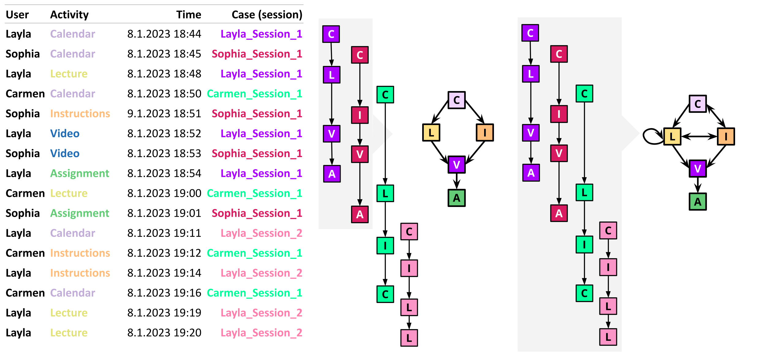
From the event log, we often construct what is known as the Directly-Follows Graph (DFG), in which we graphically represent all the activities in the event log as nodes and all the observed transitions between them as edges [5]. Figure 14.1 shows an example with event log data from students, where each case identifier represents a student’s session. First, we build the sequence of activities for each case. As such, Layla’s path for her first learning session would be: Calendar → Lecture → Video → Assignment. The path for Sophia’s first session would be: Calendar → Instructions → Video → Assignment. We put both paths together and construct a partial DFG that starts from Calendar, then it transitions either to Lecture or Instructions and then it converges back into Video and ends in Assignment. We create the paths for the remaining student sessions. Then, we combine them together through an iterative process until we have the complete graph with all the possible transitions between activities. Our final graph with the four sessions shown in Figure 14.1 would start by Calendar, then transition either to Lecture or Instructions. Then the process could transition from Lecture to Instructions or viceversa, or to Video. In addition, Lecture has a self-loop because it can trigger another lecture (see Layla’s session 2). From Video, the only possible transition is to Assignment.
In real-life scenarios, building the DFG for a complete —or large— event log may turn to be overcrowded and hard to visualize or interpret [5]. Therefore, it is common to trim activities or transitions that do not occur often. Other options include splitting the event logs by group (e.g., class sections) to reduce the granularity of the event log to be able to compare processes between groups. We can also zoom into specific parts of the course (e.g, a specific assignment or lecture) to better understand students’ activities at that time. Moreover, we can filter the event log to see cases that contain specific activities or that match certain conditions.
The DFGs are often enhanced with labels that allow us to understand the graph better. These labels are often based on the frequency of activities and transitions. For example, the nodes (representing each activity) can be labeled with the number of times (or proportion) they appear in the event data, or with the case coverage, i.e., how many cases (or what percentage thereof) they appear in. The edges (representing transitions between activities) can be labeled with the frequency of the transitions or the case coverage as well, among others. Another common way of labeling the graph is using performance measures that indicate the mean time (or median, maximum, etc.) taken by each activity and/or transition.
The DFG gives us an overarching view of the whole event log. However, in some occasions, we would like to understand the underlying process that is common to most cases of our event log. This step is called process discovery [5] and there are several algorithms to perform it such as the alpha algorithm [6], inductive techniques [7] or region-based approaches [8]. The discovered processes are then represented using specialized notation, such as Business Process Model and Notation (BPMN) [9] or Petri nets [10].
In some occasions, there are certain expectations regarding how the process should go. For instance, if we are analyzing students’ activities during a lesson, the teacher might have given a list of instructions that students are expected to follow in order. To make sure that the discovered process (i.e., what students’ data reveal) aligns with the expected process (i.e., what students were told to do in our example), conformance checking is usually performed. Conformance checking deals with comparing the discovered process with an optimal model or theorized process (i.e., an ideal process) [5]. The idea is to find similarities and differences between the model process and the real observed process, identify unwanted behavior, detect outliers, etc. As seen from our example, in educational settings, this can be used, for instance, to detect whether students are following the learning materials in the intended order or whether they implement the different phases of self-regulated learning. However, given that students are rarely asked to access learning materials in a strict sequential way, this feature has been rarely used. In the next section, we present a review of the literature on educational process mining where we discuss more examples.
3 Review of the literature
A review of the literature by Bogarín et al. [11] mapped the landscape of educational process mining and found a multitude of applications of this technique in a diversity of contexts. The most common application was to investigate the sequence of students’ activities in online environments such as MOOCs and other online or blended courses, as well as in computer-supported collaborative learning contexts [11]. One of the main aims was to detect learning difficulties to be able to provide better support for students. For example, López-Pernas et al. [12] used process mining to explore how students’ transition between a learning management system and an automated assessment tool, and identified how struggling students make use of the resources to solve their problems. Arpasat et al. [13] used process mining to study students’ activities in a MOOC, and compared the behavior of high- and low-achieving students in terms of students’ activities, bottlenecks and time performance. A considerable volume of research has studied processes where the events are instantaneous, such as clicks in online learning management systems (e.g., [14–16]). Fewer are the studies that have used activities with a start time and an end time due to the limitations in data collection in online platforms. However, this limitation has been often overcome by grouping clicks into learning sessions, as is often done in the literature on students’ learning tactics and strategies, or self-regulated learning (e.g., [12, 17–19]).
Regarding the methods used, much of the existing research is limited to calculating performance metrics and visualizing DFGs, whereby researchers attempt to understand the most commonly performed activities and the common transitions between them. For example, Vartiainen et al. [20] used video coded data of students’ participation in an educational escape room to visualize the transitions between in-game activities using DFGs. Oftentimes, researchers use DFGs to compare (visually) across groups, for example high vs. low achievers, or between clusters obtained through different methods. For instance, Saqr et al. [21] implemented k-means clustering to group students according to their online activity frequency, and used DFGs to understand the strategies adopted by the different types of learners and how they navigate their learning process. Using a different approach, Saqr and López-Pernas [22] clustered students groups according to their sequence of interactions using distance-based clustering, and then compared the transitions between different interactions among the clusters using DFGs.
Going one step further, several studies have used process discovery to detect the underlying overall process behind the observed data [11]. A variety of algorithms have been used in the literature for this purpose, such as the alpha algorithm [23], the heuristic algorithm [24], or the fuzzy miner [18]. Less often, research on educational proecss mining has performed conformance checks [11], comparing the observed process with an “ideal” or “designed” one. An example is the work by Pechenizkiy et al. [25], who used conformance checking to verify whether students answered an exam’s questions in the order specified by the teacher.
When it comes to the tools used for process mining, researchers have relied on various point-and-click software tools [11]. For example, Disco [26] has been used for DFG visualization by several articles (e.g., [27]). ProM [28] is the dominant technology when it comes to process discovery (e.g., [19, 29]) and also conformance checking (e.g., [25]). Many articles have used the R programming language to conduct process mining, relying on the bupaverse [30] framework for basic metrics and visualization (the one covered in the present chapter), although not for process discovery (e.g., [12]) since the algorithm support is scarce.
4 Process mining with R
In this section, we present a step-by-step tutorial with R on how to conduct process mining of learners’ data. First, we will install and load the necessary libraries. Then, we will present the data that we will use to illustrate the process mining method.
4.1 The libraries
As a first step, we need two basic libraries that we have used multiple times throughout the book: rio for importing the data [31], and tidyverse for data manipulation [32]. As for the libraries used for process mining, we will first rely on bupaverse, a meta-package that contains many relevant libraries for this purpose (e.g., bupaR), which will help us with the frequentist approach [30]. We will use processanimateR to see a play-by-play animated representation of our event data. You can install the packages with the following commands:
You can then load the packages using the library() function.
library(bupaverse)
library(tidyverse)
library(rio)
library(processanimateR)4.2 Importing the data
The dataset that we are going to analyze with process mining contains logs of students’ online activities in an LMS during their participation on a course about learning analytics. We will also make use of students’ grades data to compare activities between high and low achievers. More information about the dataset can be found in the data chapter of this book [33]. In the following code chunk, we download students’ event and demographic data and we merge them together into the same dataframe (df).
df <- import("https://github.com/lamethods/data/raw/main/1_moodleLAcourse/Events.xlsx")
all <- import("https://github.com/lamethods/data/raw/main/1_moodleLAcourse/AllCombined.xlsx") |>
select(User, AchievingGroup)
df <- df |> merge(all, by.x = "user", by.y = "User")When analyzing students’ learning event data, we are often interested in analyzing each learning session separately, rather than considering a longer time span (e.g., a whole course). A learning session is a sequence (or episode) of un-interrupted learning events. To do such grouping, we define a threshold of inactivity, after which, new activities are considered to belong to a new episode of learning or session. In the following code, we group students’ logs into learning sessions considering a threshold of 15 minutes (15 min. × 60 sec./min. = 900 seconds), in a way that each session will have its own session identifier (session_id). For a step-by-step explanation of the sessions, code and rationale, please refer to the sequence analysis chapter [1]. A preview of the resulting dataframe can be seen below. We see that each group of logs that are less than 900 seconds (15 minutes) apart (Time_gap column) are within the same session (new_session = FALSE) and thus have the same session_id. Logs that are more than 900 seconds apart are considered a new session (new_session = TRUE) and get a new session_id.
sessioned_data <- df |>
group_by(user) |>
arrange(user, timecreated) |>
mutate(Time_gap = timecreated - (lag(timecreated))) |>
mutate(new_session = is.na(Time_gap) | Time_gap > 900) |>
mutate(session_nr = cumsum(new_session)) |>
mutate(session_id = paste0 (user, "_", "Session_", session_nr)) |> ungroup()
sessioned_data4.2.1 Creating an event log
Now, we need to prepare the data for process mining. This is performed by converting the data into an event log. At a minimum, to construct our event log we need to specify the following:
case_id: As we have explained before, the case identifier allows to differentiate between all cases (i.e, subjects) of the process. In our dataset, since we are analyzing activities in each learning session, thecase_idwould represent the identifier of each session (the columnsession_idof our dataframe that we have just created in the previous step).activity_id: It indicates the type of activity of each event in the event log. In our dataset, we will use the columnActionthat can take the values: “Course_view”, “Assignment”, “Instructions”, “Group_work”, etc. LMS logs often contain too much granularity so it is useful to recode the events to give them more meaningful names [33].timestamp: It indicates the moment in which the event took place. In our dataset, this is represented by thetimecreatedcolumn which stores the time where each ‘click’ on the LMS took place.
Now that we have defined all the required parameters, we can create our event log. We will use the simple_eventlog() function from bupaR and supply the arguments to the function (corresponding to the aforementioned process elements) to the respective columns in our dataset.
event_log <- simple_eventlog(sessioned_data,
case_id = "session_id",
activity_id = "Action",
timestamp = "timecreated")In our example, each row in our data represents a single activity. This is often the case in online trace log data, as each activity is a mere instantaneous click with no duration. As explained earlier, in other occasions, activities have a beginning and an end, and we have several rows to represent all instances of an activity. For example, we might have a row to represent that a student has begun to solve a quiz, and another one to represent the quiz’s submission. If the data looks like that, we might need to use the activitylog() function from bupaR to create our activity log, and indicate, using the lifecycle_id argument, which column indicates whether it is the start or end of the activity, or even intermediate states.
4.2.2 Inspecting the logs
Now that we have created our event log, we can use the summary() function to get the descriptive statistics. The results show that we have a total of 95,626 events for 9,560 cases (in our example, student sessions) and 12 distinct activities (the actions in the learning management system). We have 4,076 distinct traces (i.e., unique cases), which in our example means that there are sessions that have the exact same sequence of events. These traces are, on average, 10 events long, and span from September 9th 2019 to October 27th 2019.
event_summary <- summary(event_log)Number of events: 95626
Number of cases: 9560
Number of traces: 4076
Number of distinct activities: 12
Average trace length: 10.00272
Start eventlog: 2019-09-09 14:08:01
End eventlog: 2019-10-27 19:27:41We may now inspect what the most common activities are in our event log (Table 14.1). The absolute_frequency column represents the total count of activities of each type, whereas the relative_frequency represents the percentage (as a fraction of 1) that each activity represents relative to the total count of activities. We see that the working on the group project (Group_work) is the most frequent activity (with 32,748 instances), followed by viewing the course main page (Course_view) with 25,293 instances.
activities(event_log)| Action | absolute_frequency | relative_frequency |
|---|---|---|
| Group_work | 32748 | 0.34245916 |
| Course_view | 25293 | 0.26449919 |
| Practicals | 10020 | 0.10478322 |
| Assignment | 7369 | 0.07706063 |
| Instructions | 6474 | 0.06770125 |
| General | 3346 | 0.03499048 |
| Feedback | 3114 | 0.03256437 |
| Social | 2191 | 0.02291218 |
| La_types | 1891 | 0.01977496 |
| Theory | 1377 | 0.01439985 |
| Ethics | 1028 | 0.01075021 |
| Applications | 775 | 0.00810449 |
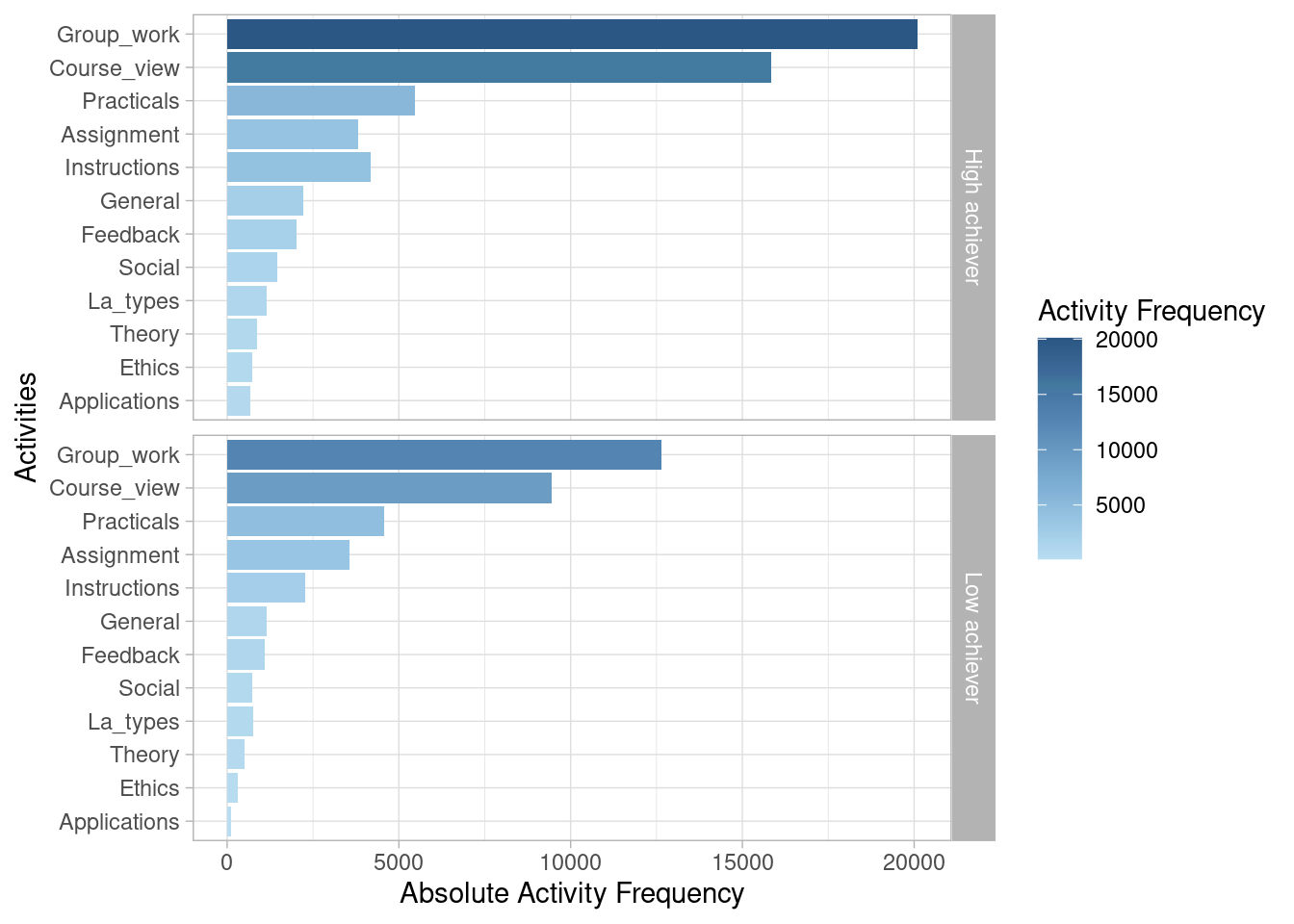
We can also view the most frequent activities in graphical form. We can even visually compare the frequency of activities between different groups (e.g., high achievers vs. low achievers).
event_log |> activity_frequency("activity") |> plot()
event_log |> group_by(AchievingGroup) |> activity_frequency("activity") |> plot()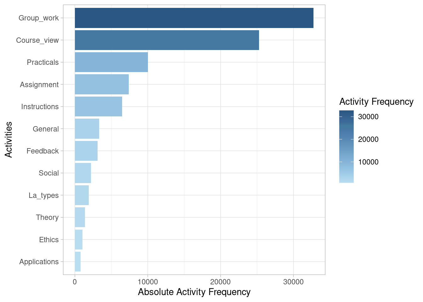
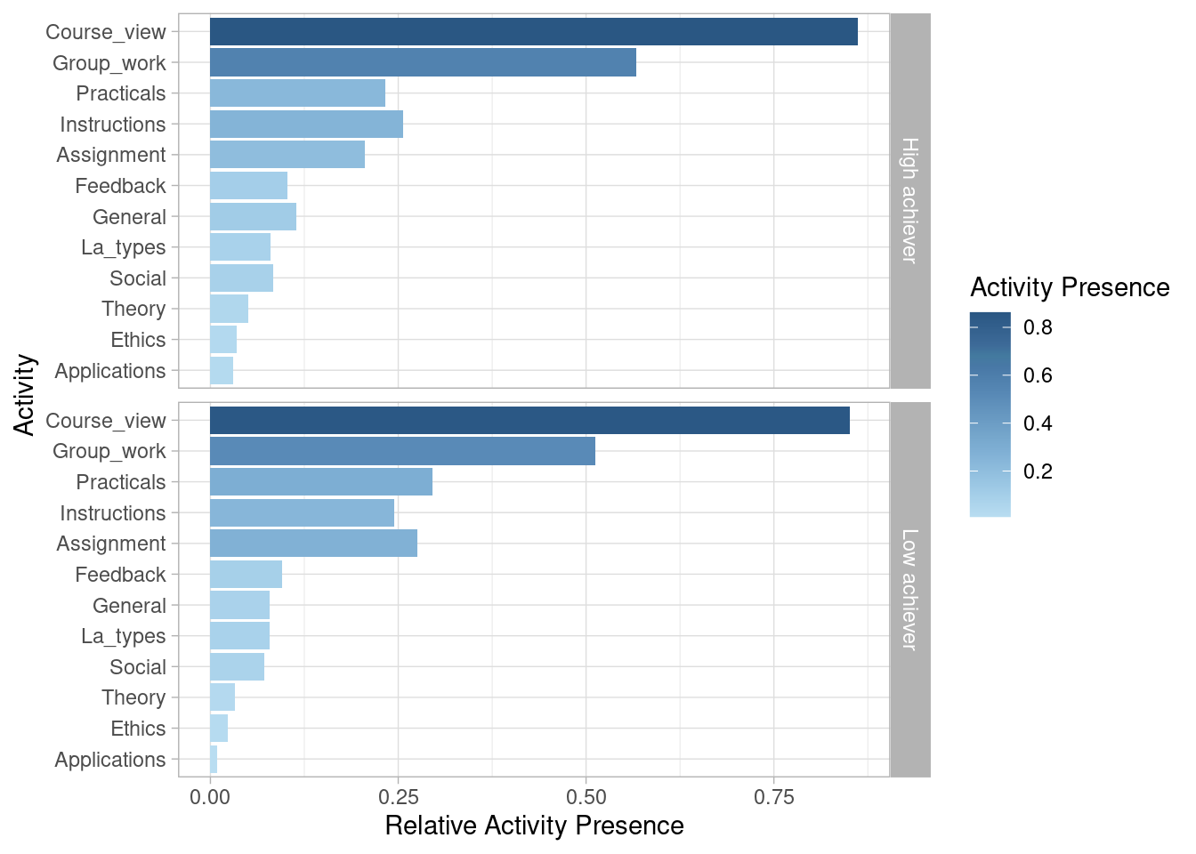
We may be also interested in looking at activity presence, also known as case coverage. This refers to the percentage of cases that contain each of the activities at least once. Most sessions (85.8%) include visiting the main page of the course (Course_view). Slightly over half (54.6%) involve working on the group project (Group_work). Around one quarter include working on the Practicals (25.7%), Instructions (25.2%), and Assignment (23.2%). Other activities are less frequent.
event_log |> activity_presence() |> plot()
event_log |> group_by(AchievingGroup) |> activity_presence() |> plot()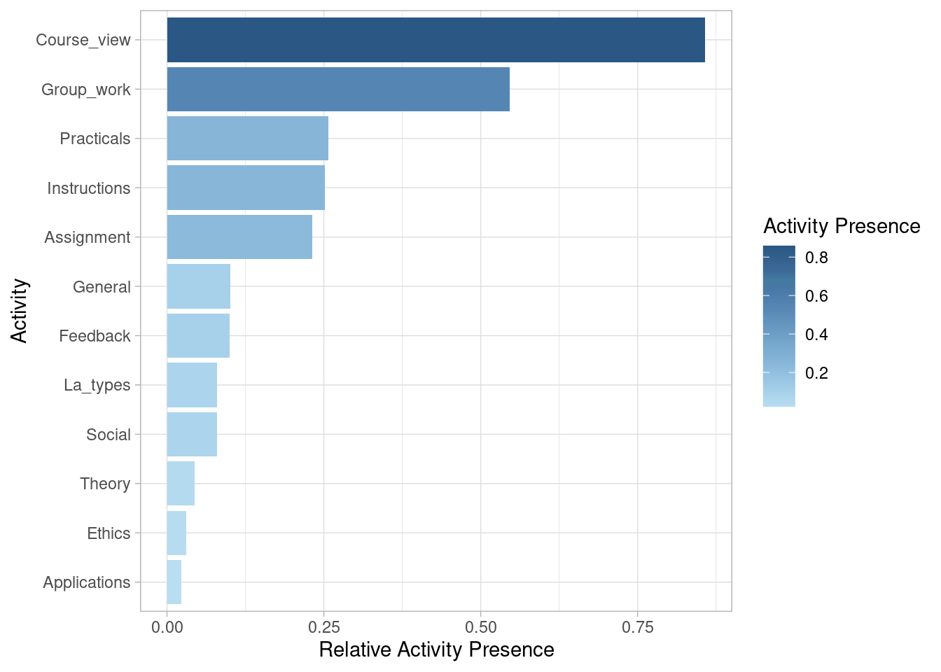
If we are interested in the transition between activities, we can plot the antecedent-consequent matrix. This visualization tells us how many transitions there has been from the activities on the left side (antecedent) to the activities on the bottom side (consequent).
event_log |> process_matrix() |> plot()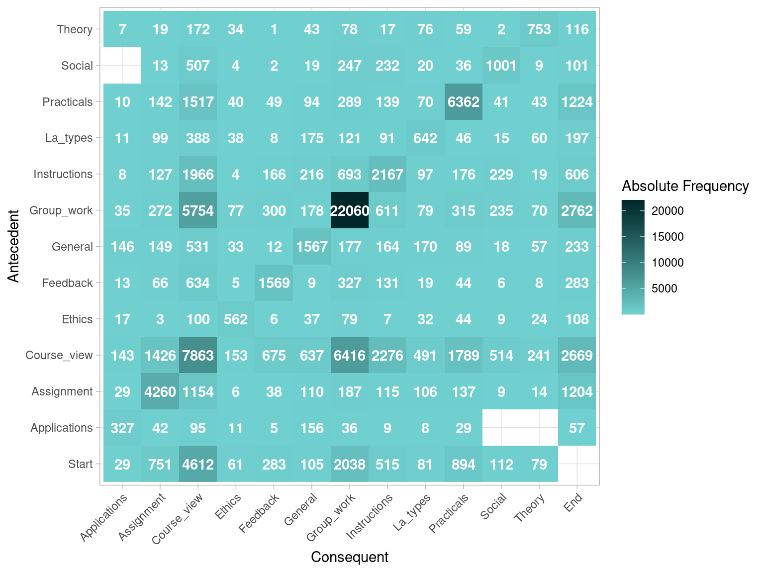
Figure 14.4 shows that there are 6416 transitions from Course_view to Group_work within the same session. The most common transition is from Group_work to more Group_work, with 22060 instances. Note that, on the antecedent side (left), there is an additional row for Start. This allows to represent the activities that occur right at the beginning as a transition from Start, since they do not have any other activity as antecedent. In this case, we see that most sessions start with Course_view (4612). On the consequent side (bottom), we see that there is an additional column on the right side for End, representing the end of a session. This allows to represent the activities that occur at the very end of a session, since they do not have any other activities following. We see that sessions are most likely to end by Group_work (2762), closely followed by Course_view (2669). Another aspect worth noting is that some cells in our matrix are empty, which represents the fact that a transition between the activity on the left, and the activity on the bottom is not present in any of the cases in our dataset. For example, we see that there are no transitions between Applications and Theory. Another —obvious— example is the cell from Start to End, as sessions should have at least one event and therefore they can never go from Start to End without any other event in the middle.
4.2.3 Visualizing the process
Now, it is time to visualize the event log using the DFG. Within the bupaverse framework this graph is referred to as process map. We can use the process_map() function for this purpose (Figure 14.5).
event_log |> process_map() By default, the process map contains every single activity and transition between activities. As the number of activities and cases increase, this can become unreadable, as is the case with our example. Therefore, we might need to trim some less frequent activities to be able to better visualize the process. We will choose to cover 80% of the activities. This means that we will select the most frequent activities in order, up to when we have accounted for 80% of all the activities in the event log. If we go back to Table 14.1, we can see that all activities ranging from the most frequent activity (Group_work) to Instructions account roughly to 80%, so we are left with the top five activities and exclude the rest. There is no standard for choosing a threshold for trimming and it is up to the researcher to define the threshold. As discussed in the introduction, such approach may yield different process maps according to the trimming threshold. A good rule of thumb for choosing this threshold is that the process map should be readable but at the same time no essential information should be removed. In our case, the activities filtered out are very infrequent and specific to certain lessons in the course, so they are not representative to the course as a whole. Another strategy would be to combine these activities into a single one such as Reading, which would allow to simplify our analysis while keeping all the information. For demonstration processes, we proceed by filtering the log and to operate with it in subsequent steps.
event_log |> filter_activity_frequency(percentage = 0.8) -> event_log_trimmedIf we now plot the process map of the trimmed event log, we will be able to see the process much more clearly (Figure 14.6). When interpreting a process map it is common to start by commenting on the nodes (the activities) and their frequency. For example, we would say that Group_work is the most frequent activity with 32,748 instances, followed by Group_work, etc., as we have already done in Table 14.1. Next, we would describe the transitions between activities, with emphasis on how sessions start. Most sessions (5,059) —in the trimmed dataset— start by viewing the course main page Course view. We can see this information on the edge (arrow) that goes from Start to Course_view. The second most common first step is Group_work (2,129). Most instances of Group_work are followed by more Group_work (22,429, as can be seen from the self-loop). The most common transitions between activities are between Course_view and Group_work, with 6,000+ instances between one another both ways, as we can infer from the labels of the edges between one another. Viewing the course main page (Course view) is the most central activity in the process map as it has multiple transitions with all the other activities, since students often use the main page to go from one activity to the next.
event_log_trimmed |> process_map() As we have seen, each node of the process contains the activity name along with its overall frequency, that is, the number of instances of that activity in our event log. Similarly, the edges (the arrows that go from activity to activity) are labeled with the number of times each transition has taken place. These are the default process map settings. Another way of labeling our process map is using the frequency("absolute-case") option, which counts the number of cases (i.e., sessions in our event log) that contain each given activity and transition (Figure 14.7). Instead of seeing the count of activities and transitions, we are seeing the count of sessions that contain each activity and transition. For example, we could say that 8,203 sessions contain the activity Course_view.
event_log_trimmed |> process_map(frequency("absolute-case"))Sometimes we may be interested in the percentage (relative proportion) rather than the overall counts because it may be easier to compare and interpret. In such a case, we can use the frequency("relative") and frequency("relative-case") options. In the former, the labels will be relative to the total number of activities and transitions (Figure 14.8 (a)), whereas in the latter, the labels will be relative to the number of cases (or proportion thereof) (Figure 14.8 (b)). For example, in Figure 14.8 (a), we see that Group_work accounts for 39.98% of the activities, whereas in Figure 14.8 (b) we see that it is present in 55.25% of the cases (i.e., sessions).
event_log_trimmed |> process_map(frequency("relative"))
event_log_trimmed |> process_map(frequency("relative-case"))We can combine several types of labels in the same process map, and even add labels related to aspects other than frequency. In the next example, we label the nodes based on their absolute and relative frequency and we label the edges based on their performance, that is, the time taken in the transition (Figure 14.9). We have chosen the mean time to depict the performance of the edges, but we could also choose median, minimum, maximum, etc. We see, for example, that the longest transition seems to be between Assingment and Group_work, in which students take on average 1.59 minutes (as seen on the edge label). The shortest transition is from Practicals to Practicals (self-loop) with 0.22 minutes on average.
event_log_trimmed |> process_map(type_nodes = frequency("absolute"),
sec_nodes = frequency("relative"),
type_edges = performance(mean))Another very useful feature is to be able to compare processes side by side. We can do so by using the group_by() function before calling process_map(). We see that the process map does not capture any meaningful difference between the two groups (Figure 14.10).
event_log_trimmed |> group_by(AchievingGroup) |> process_map(frequency("relative"))We can even reproduce the whole event log as a video using the function animate_process from processanimateR.
animate_process(event_log_trimmed)5 Discussion
We have demonstrated how to analyze event log data with process mining and how the visualization of process models can summarize a large amount of activities and produce relevant insights. Process models are powerful, summarizing, visually appealing and easy to interpret and understand. Therefore, process mining as a method has gained large scale adoption and has been used in a large number of studies to analyze all sorts of data. This chapter has offered an easy to understand overview of the basic concepts including the composition of the event log and the modelling approach that process mining undertakes. We also offered a brief overview of some examples of literature that have used the method in the analysis of students’ data. Then, a step-by-step tutorial has shown different types of visualization in the form of process maps that are based on raw frequency, relative frequency, performance (time). Later, we have shown how process maps can be used to compare between groups and show their differences. The last part of the chapter offered a guide of how to animate the process maps and see how events occur in real-time. Please note that our approach is restricted to , which is the most popular and well-maintained framework for process mining within the R environment.
Whereas we share the enthusiasm for process mining as a powerful method, we also need to discuss the method from the rigor point of view. In many ways —as we will discuss later— process mining is largely descriptive and often times exploratory. While this is acceptable in the business domain, it needs to be viewed here from the viewpoint of scientific research and what claims we can make or base on a process map. As the tutorial has already shown, several parameters and decisions have to be made by the researcher and such decisions affect the output visualizations in considerable ways (e.g., filtering the event log). The said decisions are often arbitrary with no guidance or standards to base such decisions on. So, caution has to be exercised from over interpreting the process maps that have undergone extensive filtering. In fact, most researchers have used process mining as an auxiliary or exploratory method hand-in-hand with other tools such as sequence analysis or traditional statistics. In most cases, the conclusions and inferences were based on the other rigorous methods that are used, for instance, to statistically compare two groups. One can think of the process mining described in this chapter more of a visualization tool for the most common transitions or a method for visualizing the big picture of an event log in an intuitive way.
Another known problem of process mining is that most algorithms are black-boxed (i.e., the data processing is unclear to the researcher), with no fit statistics or randomization techniques to tell if the estimated process model is different from random. The absence of confirmatory tests makes the answer to the question of whether process mining actually recover the underlying process largely speculative. Moreover, all of the tools, algorithms, and visualization techniques have been imported verbatim from the business world and therefore, their validity for educational purposes remains to be verified. In the same vein, comparing across groups is rather done descriptively, without a statistic to tell whether the observed differences are actually significant or just happened by chance. In other methods such as psychological network analysis [34], several methods are available to create randomized models that assess the credibility of each edge, the stability of centrality measures, the differences between edges as well as to compare across networks regarding each of these parameters. Given that the algorithms, and the modelling technique necessitate trimming (discarding a considerable amount of data), it is bold to assume that the remaining process map (after trimming) is a true representation of the underlying process.
It is also important to emphasize here that, given that the field name is “process mining”, the method does not translate to efficient analysis of the learning process. In fact, it is unrealistic to assume that process mining as a method —or any other method at large— can capture the full gamut of the complexity of the learning process as it unfolds across various temporal scales in different ways (e.g., transitions, variations, co-occurrence). A possible remedy for the problem lies in the triangulation of process mining models with other methods, e.g., statistics or better use a Markovian process modeling approach [3]. Stochastic process mining models (covered in detail in Chapter 12 [3]) are more advantageous theoretically and methodologically. Stochastic process mining models are theoretically robust, account for time and variable dependencies, offer fit statistics, clustering methods, several other statistics to assess the models and a wealth of possibilities and a growing repertoire of inter-operable methods.
6 Further readings
There are multiple resources for the reader to advance their knowledge about process mining. To learn more about the method itself, the reader should refer to the book Process Mining: Data Science in Action [35] and the Process Mining Handbook [36]. For more practical resources, the reader can refer to the bupaverse [30] documentation as well as find out more about the existing bupaverse extensions. The tutorial presented in this chapter has dealt with process analysis and visualization but not process discovery or conformance checking as the tools available in R are limited for these purposes. For process discovery in R, the reader can use the heuristicsMineR package [37], and for conformance checking, the pm4py package [38], a wrapper for the Python library of the same name. A practical guide with Python is also available in A Primer on Process Mining: Practical Skills with Python and Graphviz [39]. For specific learning resources on educational process mining, the reader can refer to the chapter “Process Mining from Educational Data” [40] in the Handbook of Educational Data Mining, and “Educational process mining: A tutorial and case study using Moodle data sets” [41] in the book Data Mining and Learning Analytics: Applications in Educational Research. Moreover, the reader is encouraged to read the existing literature reviews on educational process mining (e.g., [11, 42]).