
library(ggplot2)
library(patchwork)
library(dplyr)
library(caret)
library(ncvreg)
library(pROC)

repo <- "https://github.com/lamethods/data2/raw/refs/heads/main/"
dataset <- "mooc/HXPC13_DI_v3_11-13-2019.RDS"

mydata <- readRDS(url(paste0(repo, dataset)))
data <- mydata[,c("certified","course_id","explored","gender",
                  "nevents","ndays_act","nplay_video","nchapters",
                  "nforum_posts","final_cc_cname_DI")]
data[data == ""] <- NA
data <- na.omit(data)5 Comparative Analysis of Regularization Methods for Predicting Student Certification
Abstract
This chapter uses predicting student certification in online courses hosted on edX to demonstrate how to apply three powerful regularization methods, namely Least Absolute Shrinkage and Selection Operator (LASSO), Smoothly Clipped Absolute Deviation (SCAD), and Minimax Concave Penalty (MCP) in constructing a predictive model. These advanced statistical methods are especially valuable in scenarios where we have a multitude of potential predictors and need to select appropriate variables to establish viable predictive models.
1 Introduction
In the past decade, the educational landscape has undergone a seismic shift with the advent and proliferation of online learning platforms [1]. Among these, Massive Open Online Courses (MOOCs) have emerged as a transformative force, democratizing access to high-quality education on a global scale [2]. First emerged in 2008, Massive Open Online Courses (MOOCs) provide anyone with an internet connection and low-cost access to educational materials and activities delivered by experts. Like other forms of adult education, the establishment of MOOCs aims to help learners realize their potential and apply newly acquired knowledge and skills to improve their lives [3]. Students enroll in MOOCs for various reasons, including personal interest, career advancement, academic support, or social connections [4]. Unlike traditional online or in-person adult education courses, MOOCs allow students to access courses anywhere and time. Despite their potential, MOOCs have faced many challenges, such as accreditation and certification (Sanchez-Gordon), instructional design [5], types of learners [6], as well as dropout rates [7].
At the forefront of this revolution stands edX Online Courses & Programs, a pioneering platform founded in May 2012 under the administration of the Massachusetts Institute of Technology (MIT). As a leader in the MOOC space, the courses on the edX are, offered by world-renowned institutions, schools, non-profit organizations, and corporations across a diverse array of subjects, from subjects in science, technology, engineering, and math (STEM) to social sciences and humanities. edX has opened the doors of elite education to millions of learners worldwide through its commitment to accessibility and rigorous academic standards, making it a beacon of innovation in online education.
In the traditional classrooms where the teaching staff interact with students face-to-face [8], this allows them to have direct perceptions of students’ levels of engagement, hence, targeted strategies can be implemented in advance to increase student engagement and to prevent students from dropping out.
In the online context, with the advancement of learning analytics to capture large volumes of digital trace data, which are combined with various demographic data, researchers and educators can predict students’ tendency to drop out earlier in the course by applying advanced data mining and statistical techniques [9]. This also aids in understanding and improving the quality of student learning experiences [10].
One of the important indicators of student completion of online courses hosted on edX is to obtain an official certification of course. Hence, understanding factors impacting students obtaining course certification may provide course developers valuable information on strategies to improve the design of the course, online pedagogies, and methods of delivery to foster student online engagement and improve retention rate.
It shall be noted that many references like Jovanovic et al. [11] and Gray and Perkins [12] studied machine learning methods, such as random forests, to predict student course performance. However, our method differs as we focus on high-dimensional predictors and apply regularization techniques to highlight key predictors associated with learning outcome predictions. Specifically, we aim to create an elegant predictive model by using regularization to eliminate redundant predictors. Moreover, this chapter uses predicting student certification in online courses hosted on edX to demonstrate how to apply three powerful regularization methods, namely Least Absolute Shrinkage and Selection Operator (LASSO) [13], Smoothly Clipped Absolute Deviation (SCAD) [14], and Minimax Concave Penalty (MCP) [15] in constructing a predictive model. These advanced statistical methods are especially valuable in scenarios where we have a multitude of potential predictors and need to select appropriate variables to establish viable predictive models. Therefore, we aim to achieve the following objectives:
Illustrate the strengths of LASSO, SCAD, and MCP in constructing predictive models using predicting obtaining course certification in edX courses as an example. The three advanced regularization methods each have unique strengths in the process of establishing predictive models. Through applying them to a specific context – success in obtaining course certification in edX courses, it is easy to understand the relative effectiveness of these methods, providing researchers, educators, and course designers hands-on knowledge so that they can select appropriate methods by considering the unique characteristics of each method and make similar predictions of their online courses;
Uncover the key factors contributing to student certification in edX courses: We hope to identify the most key predictors of student success by analyzing a wide range of variables. This knowledge can inform both learners and educators, helping to create more effective learning strategies and support systems;
Identify the most important predictors of student success: Through variable selection and model interpretation, we aim to pinpoint the factors that strongly influence certification outcomes. This information can be invaluable for course designers, instructors, and platform developers in optimizing the online learning experience;
Provide actionable insights to inform course design and student support strategies: By understanding the key drivers of student success, we can offer evidence-based recommendations for improving course structure, content delivery, and support mechanisms on edX and similar platforms.
2 Methodologies
In this section, we will describe three regularization methods (i.e., LASSO, SCAD, and MCP) and the cross-validation method for hyperparameter tuning. In addition, we also will introduce some popular classification evaluation metrics.
2.1 Regularization Methods for High-Dimensional Data
In the context of high-dimensional data, where the number of predictors (\(p\)) is large relative to the number of observations (\(n\)), traditional statistical methods often fail due to overfitting, multicollinearity, and computational issues. Regularization methods have emerged as powerful tools to address these challenges by introducing a penalty term to the loss function, effectively shrinking some coefficient estimates towards zero and, in some cases, setting them exactly to zero [16].
These methods perform simultaneous variable selection and coefficient estimation, making them particularly useful in scenarios where identifying the most important predictors is as crucial as making accurate predictions. The general form of a penalized regression problem (with regression coefficients \(\beta\)) can be written as [17, 18]: \[\min_{\beta}\{L(\beta) + \lambda P(\beta)\}\] where \(L(\beta)\) is the loss function (e.g., negative log-likelihood for logistic regression), \(P(\beta)\) is the penalty function, and \(\lambda\) is the tuning parameter controlling the strength of regularization. Moreover, we will delve deeper into each of the three regularization methods (LASSO, SCAD, and MCP) we implemented in the following contents.
Remark. In this study, we focus on a classification task using regularization methods, specifically through three types of regularized logistic regression models. We need to adjust the first component for continuous response variables, replacing the logistic loss function with alternatives like least squares or robust losses such as Huber [19] or exponential loss [20]. Multicollinearity is not a concern in our regularization approach. Regularization methods inherently address multicollinearity by applying penalties that shrink the coefficients of correlated predictors, effectively reducing redundancy and enhancing model stability.
2.1.1 LASSO
LASSO, introduced by Tibshirani [13], adds an L1 penalty to the loss function: \[P(\beta) = ||\beta||_{1} =\Sigma |\beta_j|.\] The L1 penalty has the property of shrinking some coefficients exactly to zero, effectively performing variable selection. This is due to the geometry of the L1 ball, which intersects with the contours of the loss function at the axes, leading to sparse solutions [16]. Key properties of LASSO are listed: a) Performs both variable selection and regularization; b) Produces sparse models, which are often easier to interpret; c) Can handle high-dimensional data (\(p > n\)); and d) Tends to select one variable from a group of correlated predictors. However, LASSO has some limitations: a) In the \(p > n\) case, it selects most \(n\) variables before saturation; b) It can be biased for large coefficients; and c) It does not have the oracle property (consistent variable selection).
2.1.2 SCAD
SCAD, proposed by Fan and Li [14], is a non-convex penalty that aims to overcome some of the limitations of LASSO. The SCAD penalty is defined as: \[P(\beta) = \begin{cases} \lambda|\beta| & \text{if } |\beta| \leq \lambda \\ -\frac{\beta^2 - 2a\lambda|\beta| + \lambda^2}{2(a-1)} & \text{if } \lambda < |\beta| \leq a\lambda \\ \frac{(a+1)\lambda^2}{2} & \text{if } |\beta| > a\lambda \end{cases},\] where \(a > 2\) is a tuning parameter, often set to \(3.7\) as suggested by Fan and Li [14]. Moreover, key properties of SCAD are given as a) Overcomes the bias issue of LASSO for large coefficients; b) Possesses the oracle property (asymptotically performs as well as if the true model were known in advance); c) Produces sparse solutions; d) Continuous in \(\beta\), which leads to more stable solutions. However, SCAD also has some challenges: a) Non-convex optimization problem, which can be computationally more demanding; and b) Requires tuning of two parameters (\(\lambda\) and \(a\)).
2.1.3 MCP
MCP introduced by Zhang [15], is another non-convex penalty designed to address the limitations of LASSO. The MCP is defined as: \[P(\beta) = \begin{cases} \lambda |\beta| - \frac{\beta^2}{2\gamma} & \text{if } |\beta| \leq \gamma \lambda \\ \frac{\gamma \lambda^2}{2} & \text{if } |\beta| > \gamma \lambda \end{cases},\] where \(\gamma > 1\) is a tuning parameter controlling the concavity of the penalty. It shall be noted that some key properties of MCP are listed as a) Like SCAD, it overcomes the bias issue of LASSO for large coefficients; b) Possesses the oracle property; c) Produces sparse solutions; d) Provides a smooth transition between the region of penalization and the constant region. However, there are still challenges of MCP: a) Non-convex optimization problem; and b) Requires tuning of two parameters (\(\lambda\) and \(\gamma\)).
It shall be noted that both SCAD and MCP are part of a broader class of concave penalty functions that aim to combine the variable selection properties of L1 penalties with the unbiasedness of L2 penalties for large coefficients [21]. In practice, the choice between these methods often depends on the specific characteristics of the data and the goals of the analysis. LASSO is often preferred for its simplicity and convexity, while SCAD and MCP can provide better theoretical properties and potentially more accurate coefficient estimates, especially for large effects.
2.2 K-Fold Cross-Validation for Hyperparameter Tuning
K-Fold Cross-Validation (CV) is a widely used method for hyperparameter tuning in statistical learning, providing a robust estimate of model performance across different data subsets [22]. The process begins by setting aside an independent test set and dividing the remaining data into \(K\) equally sized folds. Hyperparameter tuning is then performed by systematically exploring a predefined hyperparameter space. For each hyperparameter combination, the model is trained on \(K-1\) folds and validated on the remaining fold, rotating through all \(K\) folds. The average performance across these \(K\) iterations is used to assess each hyperparameter set. This approach helps select hyperparameters that generalize well to unseen data, reducing overfitting risk.
The K-Fold CV process for hyperparameter tuning typically involves several steps: defining a hyperparameter grid or search space, performing the cross-validation loop for each hyperparameter combination, selecting the best-performing hyperparameters, and finally training and evaluating the model on the entire dataset and held-out test set, respectively. The hyperparameter search can be conducted using various methods, including grid search, random search [23], or more advanced techniques like Bayesian optimization [24]. While this method offers advantages such as robust performance estimation and efficient use of limited data, it also presents challenges. These include computational cost, especially for large datasets or complex models, and the potential instability of results depending on the specific folds used.
2.3 Classification Evaluation Metrics
In classification problems, especially binary classification, several metrics are commonly used to evaluate model performance. These metrics provide different perspectives on the model’s effectiveness and are derived from the confusion matrix. Understanding these metrics is crucial for properly assessing and comparing classification models. Before diving into the metrics, it is important to understand the confusion matrix in Table 1, which is the foundation for these metrics.
| Predicted Positive | Predicted Negative | |
|---|---|---|
| Actual Positive | True Positive (TP) | False Negative (FN) |
| Actual Negative | False Positive (FP) | True Negative (TN) |
Based on the confusion matrix, five popular classification measurement metrics (Accuracy, Precision, Recall, F1 score, and AUC) are derived as below [25]:
Accuracy is the proportion of correct predictions (both true positives and true negatives) among the total number of cases examined as: \[\text{Accuracy} =\frac{\text{TP} + \text{TN}}{\text{TP} +\text{ TN}+ \text{FP} + \text{FN}}.\]
Precision is the proportion of true positive predictions among all positive predictions and is formulated as: \[\text{Precision} =\frac{\text{TP}}{\text{TP}+\text{FP}}.\]
Recall is the proportion of actual positive instances that were correctly identified and is formulated as: \[\text{Recall} =\frac{\text{TP}}{\text{TP}+\text{FN}}.\]
F1 score is the harmonic mean of precision and recall, providing a single score that balances both metrics and the mathematical formula is: \[\text{F1} =\frac{2 \times ( \text{Precision}\times \text{Recall}) }{\text{Precision} +\text{Recall}}.\]
AUC (Area Under the receiver operating characteristic curve) is a performance metric that represents the probability that a randomly chosen positive instance is ranked higher than a randomly chosen negative instance. It is calculated as the area under the Receiver Operating Characteristic curve. A higher AUC value indicates better model performance in distinguishing between the classes.
It shall be noted that for imbalanced datasets, in cases where classes are imbalanced, accuracy can be misleading. For example, in a dataset with 95% negative cases and 5% positive cases, a model that always predicts negative would have 95% accuracy but would be useless for identifying positive cases. Therefore, an F1 score (or AUC) that combines Precision and Recall is suggested to measure the classification performance for imbalanced datasets.
3 Data Description and Exploratory Analysis
This section will present the dataset chosen for our illustration and conduct a preliminary exploration using basic visualization techniques.
3.1 Dataset Overview
Our dataset comes from an online learning platform and contains information about students enrolled in various courses. The key variables in our analysis include:
certified: Whether the student received certification (our target variable);course_id: Identifier for different courses;explored: Whether the student explored the course content;gender: Student’s gender;nevents: Number of events (interactions) by the student;ndays_act: Number of days the student was active;nplay_video: Number of video plays;nchapters: Number of chapters accessed;nforum_posts: Number of forum posts made by the student;final_cc_cname_DI: Student’s country name.
It is important to note that the response variable in our study is “certified”, with the other variables serving as predictors, as applied in Yuan et al. [26].
3.2 Data Preparation and Exploratory Data Analysis
We begin our analysis by loading the necessary libraries and preparing our data:
The following code snippet loads our dataset, selects the relevant columns, replaces empty strings with NA values, and removes any rows with missing data. Here, we shall notice our target of this chapter is to illustrate how to employ high-dimensionality reduction approaches for identifying key predictors (factors) relevant to the response (whether certified or not), thus we remove all the samples with missing data.
table(data$certified, data$course_id)
    HarvardX/PH207x/2012_Fall HarvardX/PH278x/2013_Spring
  0                     17671                       11006
1 1724 616table(data$certified, data$gender)
        f     m
  0 13077 15600
1 1078 1262table(data$certified, data$explored)
        0     1
  0 26027  2650
  1    60  2280
# Ensure 'course_id' is a factor
data$course_id <- as.factor(data$course_id)
# Rename specific course names
levels(data$course_id)[levels(data$course_id) ==
"HarvardX/PH207x/2012_Fall"] <- "c_id1"
levels(data$course_id)[levels(data$course_id) ==
"HarvardX/PH278x/2013_Spring"] <- "c_id2"Before diving into our predictive modeling, it is crucial to understand the distribution and relationships within our data. We use visualization techniques with two R packages “ggplot2” [27] and “patchwork” [28] to gain these insights.
# Certification rates by course
plot1 <- ggplot(data, aes(x = course_id, fill = factor(certified))) +
  geom_bar(position = "fill") +
  labs(y = "proportion", title = "course_id", fill = "certified") +
  theme(axis.text.x = element_text(angle = 45, hjust = 1),
        plot.title = element_text(hjust = 0.5))
# Certification rates by gender
plot2 <- ggplot(data, aes(x = gender, fill = factor(certified))) +
  geom_bar(position = "fill") +
  labs(y = "proportion", title = "gender", fill = "Certified") +
  theme(plot.title = element_text(hjust = 0.5))
# Certification rates by exploration status
plot3 <- ggplot(data, aes(x = explored, fill = factor(certified))) +
  geom_bar(position = "fill") +
  labs(y = "proportion", title = "explored", fill = "Certified") +
  theme(plot.title = element_text(hjust = 0.5))
# Combine the plots
combined_plot <- plot1 | plot2 | plot3
combined_plot + plot_layout(guides = 'collect')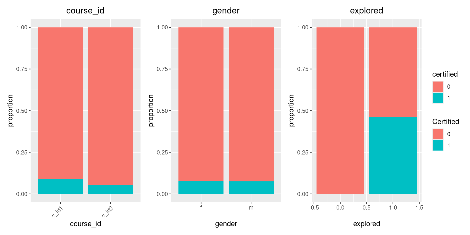
This code creates three bar plots reported in Figure 5.1 showing the certification rates by course (categorical variable), gender (binary variable), and exploration status (binary variable). These visualizations help us understand how certification rates vary across different subgroups in our dataset.
Moreover, we can obtain the detailed numerical results of the certification rates by course, gender, and exploration status with the following codes:
# course_id
table(data$certified,data$course_id)
    c_id1 c_id2
  0 17671 11006
  1  1724   616
# gender
table(data$certified,data$gender)
        f     m
  0 13077 15600
  1  1078  1262
# explored
table(data$certified,data$explored)
        0     1
  0 26027  2650
  1    60  2280
In addition, different from the former visualization for binary and categorical variables, here, we also create boxplots to visualize the relationship between certification and various numeric variables:
data_long <- data.frame(
  certified = rep(data$certified, 5),
  metric = factor(rep(c("nevents", "ndays_act", "nchapters", "nplay_video",
                        "nforum_posts"), each = nrow(data))),
  value = c(data$nevents, data$ndays_act, data$nchapters, data$nplay_video, data$nforum_posts)
)
# Create a data frame manually for faceting
faceted_plot <- ggplot(data_long, aes(x = factor(certified), y = value, fill = factor(certified))) +
  geom_boxplot() +
  facet_wrap(~ metric, scales = "free_y", ncol = 2) +
  labs(title = "Metrics by Certification Status", x = "Certified", y = "Value", fill = "Certified") +
  theme(plot.title = element_text(hjust = 0.5),
        strip.text = element_text(size = 12),
        legend.position = "bottom",
        aspect.ratio = 0.45) # Adjust the aspect ratio to make plots taller or wider

print(faceted_plot)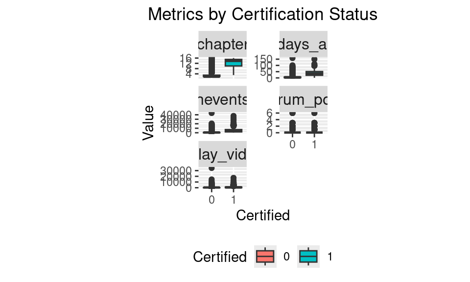
nevents, ndays_act, nchapters, nplay_video, and nforum_postsThese boxplots in Figure 5.2 reveal the differences in various engagement metrics between certified and non-certified students, highlighting that certified users generally show higher levels of engagement across multiple dimensions. In each boxplot, variables such as nevents, ndays_act, and nchapters display distinct patterns between certified and non-certified individuals, with certified students showing higher medians and wider distributions in these metrics. This pattern suggests that active and sustained participation—through frequent events, consistent activity days, and more completed chapters—is associated with a greater likelihood of certification. However, the patterns for nplay_video and nforum_posts are less clear, as both certified and non-certified students show similar distributions with low levels of forum participation overall. This lack of differentiation implies that while direct interaction with course material is crucial, forum activity and video play frequency may not significantly impact certification outcomes. Therefore, we will further analyze the visualization results with advanced regression approaches to better understand these relationships and quantify the extent to which each metric influences the likelihood of certification.
4 Data Modelling and Numerical Results
4.1 Data Preprocessing
In regularized regression for high-dimensional predictors, the optimization objective combines two components: the negative log-likelihood (for logistic regression) and the penalty function, with a hyperparameter lambda balancing them. In practice, predictors can have different scales, which may complicate the hyperparameter tuning process by impacting the search for an optimal lambda within a specified range. Therefore, it is necessary to scale the numeric variables to ensure they are on a consistent scale, improving the stability and efficiency of tuning. Additionally, converting categorical variables to factors allows the model to correctly interpret them as categorical, which is essential for meaningful analysis and accurate results. Therefore, before applying our regularization methods, we need to preprocess our data. We scale the numeric variables and convert categorical variables to factors:
data2 <- as.data.frame(scale(data[,c("nevents", "ndays_act", "nplay_video",
                                     "nchapters", "nforum_posts")]))
data2$certified <- as.factor(data$certified)
data2$course_id <- as.factor(data$course_id)
data2$explored <- as.factor(data$explored)
data2$gender <- as.factor(data$gender)
data2$final_cc_cname_DI <- as.factor(data$final_cc_cname_DI)
4.2 Model Preparation
We split our data into training (80%) and test (20%) sets:
set.seed(123)
train_indices <- createDataPartition(data2$certified, p = 0.8, list = FALSE)
train_data <- data2[train_indices, ]
test_data <- data2[-train_indices, ]
Considering the potential impacts of interactions between predictors, we construct many interaction terms in our statistical modeling. With such some interaction terms, we can clearly illustrate the effectiveness of the regularization approaches for handling high-dimensional predictors in regression modeling. We prepare our design matrices with interaction terms and response vectors:
y_train <- train_data$certified
X_train <- model.matrix(certified ~ course_id + gender + final_cc_cname_DI +
                          nevents + ndays_act +nplay_video + explored + nchapters +
                          nforum_posts + final_cc_cname_DI +
                          (course_id + nevents + ndays_act + nplay_video +
                             explored + nchapters + nforum_posts) * gender +
                          (nevents + ndays_act + nplay_video + explored +
                             nchapters + nforum_posts) * course_id,
                        data = train_data)[,-1]

y_test <- test_data$certified
X_test <- model.matrix(certified ~ course_id + gender + final_cc_cname_DI +
                         nevents + ndays_act + nplay_video + explored + nchapters +
                         nforum_posts + final_cc_cname_DI +
                         (course_id + nevents + ndays_act + nplay_video +
                            explored + nchapters + nforum_posts) * gender +
                         (nevents + ndays_act + nplay_video + explored +
                            nchapters + nforum_posts) * course_id,
                       data = test_data)[,-1]
4.3 Cross-validation and Model Fitting
We implement three regularization methods: LASSO, SCAD, and MCP. These methods are particularly useful for high-dimensional data where we have a large number of predictors relative to the number of observations. They perform variable selection by shrinking some coefficients to exactly zero, effectively removing those predictors from the model. We implement these methods using the “ncvreg” package [29] in R.
We use k-fold cross-validation to select the optimal regularization parameter (lambda) for each method with the folder number \(5\). Our implementation uses the Area Under the ROC Curve (AUC) as the performance metric:
# Function to perform cross-validation using AUC and fit the model
cv_and_fit_auc <- function(X, y, penalty, nfolds = 5) {
  set.seed(123)  # for reproducibility
  # Fit the model using the entire path
  fit <- ncvreg(X, y, family = "binomial", penalty = penalty, standardize = FALSE)
  # Perform k-fold cross-validation
  folds <- sample(rep(1:nfolds, length.out = length(y)))
  aucs <- matrix(0, nrow = nfolds, ncol = length(fit$lambda))

  for (i in 1:nfolds) {
    test_indices <- which(folds == i)
    X_train_cv <- X[-test_indices, ]
    y_train_cv <- y[-test_indices]
    X_test_cv <- X[test_indices, ]
    y_test_cv <- y[test_indices]
    # Fit model on training data
    cv_fit <- ncvreg(X_train_cv, y_train_cv, family = "binomial",
                     penalty = penalty, lambda = fit$lambda,standardize = FALSE)
    # Calculate AUC for each lambda
    for (j in 1:length(cv_fit$lambda)) {
      beta <- coef(cv_fit)[, j]
      # Ensure beta is a numeric vector
      beta <- as.numeric(beta)
      # Initialize vector to store probabilities
      probs <- numeric(nrow(X_test_cv))
      # Loop over each row in X_test_cv
      for (k in 1:nrow(X_test_cv)) {
        # Extract the predictor vector for the current row
        x_row <- X_test_cv[k, , drop = FALSE]
        # Calculate the linear predictor (including intercept)
        linear_predictor <- cbind(1, x_row) %*% beta
        # Calculate the predicted probability
        probs[k] <- 1 / (1 + exp(-linear_predictor))
      }
      # Calculate AUC for the current lambda
      roc_curve <- roc(y_test_cv, probs, quiet = TRUE)
      aucs[i, j] <- auc(roc_curve)
    }
  }
  # Calculate mean AUCs across folds
  mean_aucs <- colMeans(aucs)
  # Determine the optimal lambda
  optimal_lambda_index <- which.max(mean_aucs)
  optimal_lambda <- fit$lambda[optimal_lambda_index]
  # Extract coefficients at the optimal lambda
  coef <- coef(fit)[, optimal_lambda_index]
  return(list(fit = fit, coef = coef, optimal_lambda = optimal_lambda,
              mean_aucs = mean_aucs))
}
The cv_and_fit_auc() function performs cross-validation and model fitting to select an optimal regularization parameter (lambda) using AUC as the performance metric. We first fit a model across a range of lambda values using the ncvreg function, which applies a penalized regression technique. The data is split into nfolds subsets for cross-validation, wherein each fold, the function trains a model on the training data and evaluates it on the test data. The AUC for each value of lambda is calculated by looping through the test set and computing predicted probabilities, which are then used to generate the ROC curve. After calculating the mean AUC across all folds for each lambda, the optimal lambda is selected based on the highest average AUC. The function returns the fitted model, the coefficients at the optimal lambda, the selected lambda, and the mean AUCs across folds, providing an effective method for model tuning and evaluation.
We then fit our models with cv_and_fit_auc() function:
lasso_results <- cv_and_fit_auc(X_train, y_train, "lasso")
scad_results <- cv_and_fit_auc(X_train, y_train, "SCAD")
mcp_results <- cv_and_fit_auc(X_train, y_train, "MCP")
It shall be noted that the computational efficiency of the model fitting depends on the sample size and the dimensionality of the predictors. To speed up the fitting process, some parallel computing techniques are suggested.
4.4 Results
We evaluate our models on the test set using various performance metrics. The function calculate_test_performance() evaluates a binary classification model’s performance by taking model coefficients (coef), test predictors X_test, and true labels (y_test) as inputs. First, we ensure the data formats and dimensions are correct. Then, we calculate linear predictor values and use the logistic function to compute predicted probabilities for each test instance. These probabilities are converted to binary predictions using a threshold of 0.5. Next, the function computes various performance metrics, including accuracy, precision, recall, and F1 score using a confusion matrix, as well as the AUC using the ROC curve to measure the model’s ability to distinguish between classes. Finally, all calculated metrics are returned in a list for easy interpretation, providing a comprehensive evaluation of the model’s predictive performance.
# Function to calculate test performance metrics
calculate_test_performance <- function(coef, X_test, y_test) {
  # Ensure X_test is a matrix
  X_test <- as.matrix(X_test)
  # Ensure coef is a numeric vector
  coef <- as.numeric(coef)
  # Check that coef length matches the number of columns in X_test + 1
  # (for the intercept)
  if (length(coef) != (ncol(X_test) + 1)) {
    stop("Length of coef must be equal to the number of predictors
         plus one for the intercept.")
  }
  # Initialize vectors to store linear predictors and probabilities
  linear_predictors <- numeric(nrow(X_test))
  probs <- numeric(nrow(X_test))
  # Loop over each row in X_test
  for (i in 1:nrow(X_test)) {
    # Extract the predictor vector
    x_row <- X_test[i, , drop = FALSE]
    # Calculate the linear predictor (including intercept)
    linear_predictors[i] <- cbind(1, x_row) %*% coef
    # Calculate the predicted probability
    probs[i] <- 1 / (1 + exp(-linear_predictors[i]))
  }
  # Convert probabilities to binary predictions
  predictions <- ifelse(probs > 0.5, 1, 0)
  # Calculate performance metrics
  confusion <- confusionMatrix(factor(predictions), factor(y_test))
  accuracy <- confusion$overall['Accuracy']
  precision <- confusion$byClass['Pos Pred Value']
  recall <- confusion$byClass['Sensitivity']
  f1_score <- 2 * (precision * recall) / (precision + recall)
  # Calculate AUC
  roc_curve <- roc(y_test, probs, quiet = TRUE)
  auc <- auc(roc_curve)
  return(list(accuracy = accuracy, precision = precision, recall = recall,
              f1_score = f1_score, auc = auc))
}
Now, we employ the function calculate_test_performance() with parameter estimates from three different regularization methods.
# Calculate test performance for each method
lasso_performance <- calculate_test_performance(lasso_results$coef, X_test, y_test)
scad_performance <- calculate_test_performance(scad_results$coef, X_test, y_test)
mcp_performance <- calculate_test_performance(mcp_results$coef, X_test, y_test)
Let’s compare the performance of our three models on the test set:
Test Performance Metrics:
--------------------------------------------------------
LASSO:
Accuracy:  0.9234694
Precision: 0.8973384
Recall:    0.7744361
F1 Score:  0.8314607
AUC:       0.9508162

SCAD:
Accuracy:  0.9210204
Precision: 0.8888889
Recall:    0.7744361
F1 Score:  0.8278146
AUC:       0.9502024

MCP:
Accuracy:  0.9210204
Precision: 0.8888889
Recall:    0.7744361
F1 Score:  0.8278146
AUC:       0.9502024
All three models perform well, with accuracy above 92% and AUC above 0.95. LASSO slightly outperforms SCAD and MCP in terms of accuracy and AUC, while all three models have the same recall. The high AUC values indicate that all models are good at distinguishing between certified and non-certified students. Furthermore, one of the key advantages of these regularization methods is their ability to perform variable selection. Let’s compare which variables were selected by each method:
# Compare selected variables
compare_selection <- function(lasso, scad, mcp) {
  all_vars <- unique(c(names(lasso), names(scad), names(mcp)))
  selection <- data.frame(Variable = all_vars,
          LASSO = ifelse(all_vars %in% names(lasso)[lasso != 0], "Selected", ""),
          SCAD = ifelse(all_vars %in% names(scad)[scad != 0], "Selected", ""),
          MCP = ifelse(all_vars %in% names(mcp)[mcp != 0], "Selected", ""))
  return(selection)
}

variable_selection <- compare_selection(lasso_results$coef,
                                        scad_results$coef,
                                        mcp_results$coef)
# Print the first 5 rows of the variable_selection data frame
print(head(variable_selection, 5))
Here, we output the first 5 rows of the variable selection by using these three regularization methods where empty means unselected:
This comparison reveals which predictors are considered important by each method, and the whole results are reported in Table 9.2.
| Variable | LASSO | SCAD | MCP | |
|---|---|---|---|---|
| 1 | (Intercept) | Selected | Selected | Selected |
| 2 | course_idc_id2 | Selected | Selected | |
| 3 | genderm | |||
| 4 | final_cc_cname_DIBangladesh | |||
| 5 | final_cc_cname_DIBrazil | Selected | Selected | |
| 6 | final_cc_cname_DICanada | Selected | ||
| 7 | final_cc_cname_DIChina | Selected | ||
| 8 | final_cc_cname_DIColombia | Selected | ||
| 9 | final_cc_cname_DIEgypt | Selected | ||
| 10 | final_cc_cname_DIFrance | Selected | ||
| 11 | final_cc_cname_DIGermany | Selected | ||
| 12 | final_cc_cname_DIGreece | Selected | ||
| 13 | final_cc_cname_DIIndia | Selected | Selected | Selected |
| 14 | final_cc_cname_DIIndonesia | |||
| 15 | final_cc_cname_DIJapan | |||
| 16 | final_cc_cname_DIMexico | |||
| 17 | final_cc_cname_DIMorocco | |||
| 18 | final_cc_cname_DINigeria | Selected | Selected | Selected |
| 19 | final_cc_cname_DIOther Africa | |||
| 20 | final_cc_cname_DIOther East Asia | |||
| 21 | final_cc_cname_DIOther Europe | Selected | ||
| 22 | final_cc_cname_DIOther Middle East/Central Asia | |||
| 23 | final_cc_cname_DIOther North & Central Amer., Caribbean | Selected | ||
| 24 | final_cc_cname_DIOther Oceania | Selected | ||
| 25 | final_cc_cname_DIOther South America | |||
| 26 | final_cc_cname_DIOther South Asia | |||
| 27 | final_cc_cname_DIPakistan | Selected | Selected | |
| 28 | final_cc_cname_DIPhilippines | Selected | ||
| 29 | final_cc_cname_DIPoland | |||
| 30 | final_cc_cname_DIPortugal | Selected | Selected | |
| 31 | final_cc_cname_DIRussian Federation | Selected | ||
| 32 | final_cc_cname_DISpain | Selected | Selected | Selected |
| 33 | final_cc_cname_DIUkraine | Selected | ||
| 34 | final_cc_cname_DIUnited Kingdom | |||
| 35 | final_cc_cname_DIUnited States | Selected | ||
| 36 | final_cc_cname_DIUnknown/Other | Selected | ||
| 37 | nevents | Selected | Selected | Selected |
| 38 | ndays_act | Selected | Selected | Selected |
| 39 | nplay_video | Selected | Selected | Selected |
| 40 | explored1 | Selected | Selected | |
| 41 | nchapters | Selected | Selected | Selected |
| 42 | nforum_posts | Selected | ||
| 43 | course_idc_id2:genderm | |||
| 44 | genderm:nevents | |||
| 45 | genderm:ndays_act | Selected | ||
| 46 | genderm:nplay_video | |||
| 47 | genderm:explored1 | |||
| 48 | genderm:nchapters | Selected | ||
| 49 | genderm:nforum_posts | |||
| 50 | course_idc_id2:nevents | Selected | Selected | Selected |
| 51 | course_idc_id2:ndays_act | Selected | ||
| 52 | course_idc_id2:nplay_video | Selected | Selected | Selected |
| 53 | course_idc_id2:explored1 | Selected | Selected | |
| 54 | course_idc_id2:nchapters | Selected | ||
| 55 | course_idc_id2:nforum_posts | Selected |
Moreover, we can obtain the number of selected variables:
num_vars <- c(sum(lasso_results$coef != 0) - 1,
              sum(scad_results$coef != 0) - 1,
              sum(mcp_results$coef != 0) - 1)
cat("\nNumber of selected variables:\n")
cat("LASSO:", num_vars[1], "\n")
cat("SCAD:", num_vars[2], "\n")
cat("MCP:", num_vars[3], "\n")
This comparison shows how aggressive each method is in terms of variable selection. Typically, LASSO tends to select more predictors than SCAD and MCP, which are often more aggressive in their variable selection.
Based on the provided results, the MCP method demonstrates superior performance in variable selection while maintaining competitive predictive accuracy. MCP selected only 10 variables, significantly fewer than LASSO (36) and SCAD (14), indicating its effectiveness in achieving a more parsimonious model. Despite using fewer predictors, MCP matched SCAD’s performance across all metrics (Accuracy: 0.9210, Precision: 0.8889, Recall: 0.7744, F1 Score: 0.8278, AUC: 0.9502) and was only marginally behind LASSO in accuracy and AUC. This suggests that MCP effectively identified the most influential predictors, resulting in a simpler model with comparable predictive power. The ability to achieve such performance with fewer variables highlights MCP’s strength in balancing model complexity and predictive accuracy, making it the preferable choice for this dataset.
Remark. It shall be noted that although the original dataset contained only 10 variables, we constructed an additional 45 interaction terms for our modeling, which increased the dimensionality. As shown in Table 2, all three regularization methods effectively shrank redundant predictors to zero, with the MCP method being particularly efficient, retaining only 10 predictors. This demonstrates the effectiveness of regularization for variable selection in educational data modeling. It is also important to note that regularization methods tend to be even more effective when the number of predictors significantly exceeds the sample size, especially in extremely high-dimensional settings.
4.5 Implications for Online Learning
The Minimax Concave Penalty (MCP) method identified 10 key predictors for online learning outcomes, offering a concise yet comprehensive model. These predictors reflected the critical role of student engagement, including metrics such as total events, active days, video plays, and chapters accessed. The model also highlighted specific country effects of India, Nigeria, and Spain, suggesting that geographical or cultural backgrounds had an impact on learning outcomes. Notably, the interaction terms between course ID and engagement metrics were selected, indicating that the impact of student engagement varies across different courses. This parsimonious selection of variables provides valuable insights into the most significant factors affecting online learning success.
These findings have important implications for online education stakeholders. The results underscore the necessity of promoting active participation and regular interaction with course content, particularly video lectures. The model suggests that tailored approaches may be beneficial for students from specific countries, addressing unique challenges or leveraging strengths associated with these geographical contexts. The variation in engagement effects across courses indicates that customized strategies for course design and student support could be more effective than a uniform approach. Interestingly, the absence of demographic variables like gender in the final model implies that engagement metrics are more predictive of success than these demographic variables in this context. These insights can guide educators, course designers, and platform developers to embed desirable elements (e.g., gamification or animation) into video lectures to improve students’ online engagement [30, 31], which may, in turn, help students from diverse geographical regions to complete the course successfully.
5 Conclusion
This chapter has made significant progress in understanding the dynamics of student success in online education, particularly within the edX platform. Through our quantitative analysis employing LASSO, SCAD, and MCP regularization methods, we have successfully identified key factors contributing to obtaining certification in edX courses. The comparative evaluation of these advanced regularization techniques has highlighted their respective strengths in this context, which researchers can easily adapt to construct predictive models for similar contexts in online education.
Our findings have identified the most crucial predictors of student success, emphasizing key aspects of student engagement, course design, and geographical factors. These insights provide practical guidance for course design and student support. By applying these evidence-based results, course designers, instructors, and platform developers can enhance the online learning experience and potentially improve student outcomes and certification rates. This study lays a strong foundation for optimizing digital learning platforms and supporting diverse learners worldwide as online education evolves.
Furthermore, in the field of education, regularization methods can help researchers identify the most influential factors impacting various cognitive (e.g., academic achievement, development of generic skills) and affective learning outcomes (e.g., learning engagement, course satisfaction, motivation in learning), even when dealing with numerous potential predictors. In particular, regularization methods are useful in understanding learners’ experiences in online/blended learning via selecting key factors from the large volume of observational data, which records detailed and nuanced learner behaviors in a time-stamped manner.
References
1.
Papadakis S (2023) MOOCs 2012-2022: An overview. Advances in Mobile Learning Educational Research 3:682–693
2.
Deng R, Benckendorff P, Gannaway D (2019) Progress and new directions for teaching and learning in MOOCs. Computers & Education 129:48–60
3.
Knowles MS (1970) The Modern Practice of Adult Education: Andragogy versus Pedagogy. Englewood Cliffs, NJ: Cambridge Adult Education
4.
Brooker A, Corrin L, De Barba P, Lodge J, Kennedy G (2018) A tale of two MOOCs: How student motivation and participation predict learning outcomes in different MOOCs. Australasian Journal of Educational Technology 34:
5.
Spector JM, Johnson TE, Young PA (2014) An editorial on research and development in and with educational technology. Educational Technology Research and Development 62:1–12
6.
Bingol I, Kursun E, Kayaduman H (2020) Factors for success and course completion in massive open online courses through the lens of participant types. Open Praxis 12:223–239
7.
Xiong Y, Li H, Kornhaber ML, Suen HK, Pursel B, Goins DD (2015) Examining the relations among student motivation, engagement, and retention in a MOOC: A structural equation modeling approach. Global Education Review 2:23–33
8.
Han F, Ellis RA (2023) Self-reported and digital-trace measures of computer science students’ self-regulated learning in blended course designs. Education and Information Technologies 28:13253–13268
9.
Han F, Ellis RA, Pardo A (2022) The descriptive features and quantitative aspects of students’ observed online learning: How are they related to self-reported perceptions and learning outcomes? IEEE Transactions on Learning Technologies 15:32–41
10.
Siemens G, Gasevic D (2012) Guest editorial-learning and knowledge analytics. Journal of Educational Technology & Society 15:1–2
11.
Jovanovic J, López-Pernas S, Saqr M (2024) Predictive modelling in learning analytics: A machine learning approach in R. In: Learning analytics methods and tutorials: A practical guide using r. Springer Nature Switzerland Cham, pp 197–229
12.
Gray CC, Perkins D (2019) Utilizing early engagement and machine learning to predict student outcomes. Computers & Education 131:22–32
13.
Tibshirani R (1996) Regression shrinkage and selection via the LASSO. Journal of the Royal Statistical Society Series B: Statistical Methodology 58:267–288
14.
Fan J, Li R (2001) Variable selection via nonconcave penalized likelihood and its oracle properties. Journal of the American Statistical Association 96:1348–1360
15.
Zhang C-H (2010) Nearly unbiased variable selection under minimax concave penalty. The Annals of Statistics 894–942
16.
Hastie T, Tibshirani R, Wainwright M (2015) Statistical learning with sparsity. Monographs on Statistics and Applied Probability 143:8
17.
Fu L, Wang Y-G, Wu J (2024) Recent advances in longitudinal data analysis. Modeling and Analysis of Longitudinal Data 50:173
18.
Wang Y-G, Wu J, Hu Z-H, McLachlan GJ (2023) A new algorithm for support vector regression with automatic selection of hyperparameters. Pattern Recognition 133:108989
19.
Huber PJ (1973) Robust regression: Asymptotics, conjectures and Monte Carlo. The Annals of Statistics 799–821
20.
Jiang Y, Wang Y-G, Fu L, Wang X (2019) Robust estimation using modified Huber’s functions with new tails. Technometrics 61:111–122
21.
Zou H, Li R (2008) One-step sparse estimates in nonconcave penalized likelihood models. The Annals of Statistics 36:1509
22.
Hastie T, Tibshirani R, Friedman JH, Friedman JH (2009) The Elements of Statistical Learning: Data mining, Inference, and Prediction. Springer
23.
Bergstra J, Bengio Y (2012) Random search for hyper-parameter optimization. Journal of Machine Learning Research 13:
24.
Snoek J, Larochelle H, Adams RP (2012) Practical Bayesian optimization of machine learning algorithms. Advances in Neural Information Processing Systems 25:
25.
Hand DJ (2012) Assessing the performance of classification methods. International Statistical Review 80:400–414
26.
Yuan J, Qiu X, Wu J, Guo J, Li W, Wang Y-G (2024) Integrating behavior analysis with machine learning to predict online learning performance: A scientometric review and empirical study. arXiv preprint arXiv:240611847
27.
Wickham H (2011) ggplot2. Wiley Interdisciplinary Reviews: Computational Statistics 3:180–185
28.
Pedersen TL (2019) Package “patchwork.” R package http://CRAN R-project org/package= patchwork Cran
29.
Breheny P, Breheny MP (2024) Package “ncvreg”
30.
Chans GM, Portuguez Castro M (2021) Gamification as a strategy to increase motivation and engagement in higher education chemistry students. Computers 10:132
31.
Looyestyn J, Kernot J, Boshoff K, Ryan J, Edney S, Maher C (2017) Does gamification increase engagement with online programs? A systematic review. PloS One 12:e0173403