21  Detecting Long-Memory Psychological Processes in Academic Settings Using Whittle’s Maximum Likelihood Estimator: An Application with R

Abstract

Person-specific approaches are best suited to account for the complex, dynamic, and idiosyncratic processes from which cognitive, emotional, motivational, relational, and behavioral patterns emerge. Among these approaches, Whittle’s approximation of the Maximum Likelihood Estimator (MLE) enables the detection of long-term memory processes in relatively short time series of data. In this chapter, we outline the principles of Whittle’s MLE, illustrate its application—using R—to the motivational dynamics of approach and avoidance in an academic context, and then discuss the theoretical and practical implications of detecting long-memory processes in the field of education and learning.

1 Introduction

People’s cognitive, emotional, motivational, relational, and behavioral patterns emerge from complex, dynamic, and idiosyncratic processes [1]. Thus, these processes operate in an original way, at an individual level which is the most relevant scale for examining them [2]. This requires person-specific methods, particularly those based on the analysis of time series of idiographic data [3]. Some of these analysis techniques, such as the popular Detrended Fluctuation Analysis (DFA; [4]), can be used to detect whether a variable of interest is randomly fluctuating (white noise¹), or follows a movement deviating from its trajectory under the influence of random shocks (Brownian motion²), or obey particular auto-correlation structures that are redundant across different time scales and that reveal a kind of memory process in the form of a long-term dependency (1/\(f\) noise or pink noise³).

In addition to its ease of implementation, DFA has the advantage of being applicable to either stationary (e.g., white noise, pink noise) or non-stationary signals (Brownian motion). This method is based on a statistical property of fractional Brownian motion [5] whereby the size of the variance to the power \(𝛼\) is proportional to the sample size. The power value \(𝛼\) is the fractal exponent which provides information about the fluctuation structure of the variable of interest. When \(𝛼\) is between 0 and 1, the time series is stationary and can be qualified as noise. From 0 to 0.5, the time series is anti-correlated to itself, which means that an increase in the value of the variable is followed by a decrease and vice versa. At 0.5 the series corresponds to white Gaussian noise. From 0.5 to 1 the time series is autocorrelated and displays long-term memory properties. For a \(𝛼\) between 1 and 2, the series is non-stationary and is referred to as motion. A value of 1.5 corresponds to ordinary Brownian motion [6].

Despite its great popularity, DFA suffers from reliability issues when confronted with certain empirical data, particularly when the length of the time series to be analyzed is less than 500 data points. Depending on the size and target population of the studies for which this method is to be applied, it may prove very difficult to obtain such series lengths. For example, if we want to analyze walking, 500 steps represent between 10 and 12 minutes of walking, which is difficult to achieve for elderly adults with a loss of autonomy [7].

Some methods make it possible to estimate the fractal exponent of shorter time series without being affected by the estimation biases that DFA presents for such series [7–10]. This chapter presents one of these methods: Whittle’s approximation of the Maximum Likelihood Estimator (MLE). Whereas the DFA output is estimated via linear regression, Whittle’s estimator is a more sophisticated method that consists of solving an optimization problem [11]. As a comparison, with only 128 data points, Whittle’s MLE gives results twice as accurate as the DFA on 512 data points [10], the latter offering results that were however already considered satisfactory [12].

The first part of the chapter is devoted to the presentation of the principles of Whittle’s MLE, as well as their formal implementation. Next, a concrete application of Whittle’s MLE to the study of the dynamics of approach and avoidance motivation in an academic context is offered as an illustration of these principles. This illustration begins with a presentation of the motivational model referred to, continues with the application of Whittle’s MLE to a time series of individual data relating to this model, and ends with a discussion of the result obtained. The chapter concludes with an attempt to reconcile variable-centered nomothetic approaches with person-specific approaches. This reconciliation, potentially capable of resolving the ergodicity issue in psychological science, requires the primacy of person-specific approaches.

2 Principles of Whittle’s Maximum Likelihood Estimator (MLE)

The general principle of Whittle’s estimator is to find the value of \(𝛼\) in the interval [0,1] that maximizes the Whittle’s log-likelihood function accounted for by Equation 1:

\[ l_w(\alpha) = -\frac{2}{N} \sum_{j=1}^{m} \left( \ln cT'(\omega_j; \alpha) + \frac{P(\omega_j)}{cT'(\omega_j; \alpha)} \right),\tag{1} \]

where \(P(\omega_j)\) is the periodogram of the time series \(x(j)\) of length \(N\); \(\omega_j\) are Fourier’s frequencies defined as \(\omega = 2\pi j/N\); \(m\) is the integer part of \((N-1)/2\); \(T'(\omega_j; \alpha)\) is the theoretical spectral density; and \(c\) is a constant used to adjust the powers of the theoretical spectrum.

In this chapter, we will use the theoretical power spectral density of an ARFIMA (Autoregressive Fractionally Integrated Moving Average⁴) model, which enables the modeling of time series with long memory. ARFIMA models are denoted ARFIMA(\(p\),\(d\),\(q\)) with \(p\) as the order indicating the number of time lags of the autoregressive model, \(q\) as the order of the moving-average model, and \(d\) as the fractional integration parameter ranging from -0.5 to 0.5. It corresponds to the exponent \(𝛼\) via the conversion: \(𝛼\) = \(d\) + ½ with \(𝛼\) belonging to the interval [0, 1]. The theoretical power spectral density that is used here is that of the ARFIMA(0,\(d\),0) model, which reads as follow:

\[ T'(\omega_j; \alpha) = \frac{1}{2\pi} \left( 2 \sin \frac{\omega_j}{2} \right)^{1-2\alpha}. \tag{2} \]

An algorithm based on Whittle’s estimator can be developed in three steps. The first one combines data pre-processing, via normalization of the time series and then estimation of the periodogram of this series. The second step is the estimation of \(α\). An optimization algorithm is used to find the \(α\) value for which the Whittle’s log-likelihood function, \(l_w(\alpha)\), reaches its maximum value. The third step is optional and is carried out only if the \(α\) value obtained from the algorithm is that of the upper bound. In this case, the maximum of the \(l_w(\alpha)\) function can be considered to belong to the interval [1,2], which means that the time series is probably non-stationary. Indeed, the \(l_w(\alpha)\) function is only applicable for stationary signals, with an \(𝛼\) value within the interval [0,1]. Nevertheless, non-stationary series can be analyzed by using a differentiated (derivative) version of the original series and then adding 1 to the \(𝛼\) value provided by the algorithm [13]. In summary, the third step consists of differentiating the time series, then applying the first two steps and finally adding 1 to the \(𝛼\) value obtained from the algorithm.

3 Application of Whittle’s MLE to motivational dynamics in an academic context

3.1 The dynamical model of approach and avoidance motivation in achievement contexts

Motivational states regarding a goal to be achieved are properties emerging from complex dynamical systems. As such, motivational states fluctuate non-linearly, thus exhibiting various patterns such as persistence of effort or its absence, as well as oscillations and even abrupt shifts between motivated and unmotivated states [14–16]. We will illustrate how Whittle’s MLE can help characterize the dynamics and the complexity of approach and avoidance motivations in an academic context, more specifically with respect to a Ph.D. student’s pursuit of the goal of reaching the defense of their doctoral thesis.

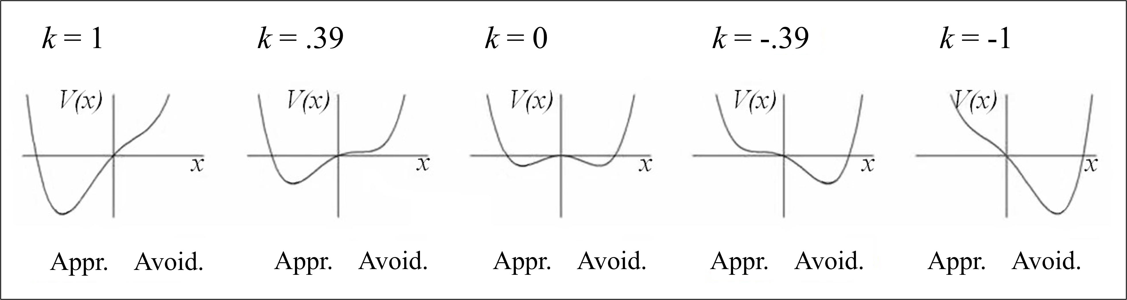
Based on the complex dynamical system perspective, approach and avoidance motivational states can be conceptualized as being constrained by two competing attractors [15]. Attractors are sets of states of a system that are more or less strongly attracted and stabilized within a limited number of values, as if—metaphorically—the trajectories of these states (here, the motivational states) were constrained by the valleys of a hilly landscape. According to Tuller et al. [17], the shape of a landscape that may include one or two attractors can be accounted for by the following equation:

\[ V(x) = kx - \frac{1}{2} x^2 + \frac{1}{4} x^4, \tag{3} \]

where \(V(x)\) is the potential function that constrains the different motivational states \(x\); \(k\) is the control parameter that specifies the direction and degree of tilt of the graph of \(V(x)\) towards approach (when \(k\) tends towards +1) and avoidance (when \(k\) tends towards –1) motivations (see Figure 1).

Approach (Appr.) and avoidance (Avoid.) attractor landscapes as defined by Equation 3 with different values of the control parameter \(k\) (from +1 to –1).

The value of the parameter \(k\) is itself conceived as resulting from the combination of three social cognitive variables considered to be necessary and sufficient for achievement motivation: Competence expectancies with regard to a goal (e.g., [18]), as well as the benefit to the self that the prospect of achieving a goal conveys and the threat to the self associated with the prospect of failure (e.g., [19]). These three variables contribute to determining \(k\) according to Equation 4:

\[ k = (Ce \times Bs) - [Ts \times (1 - Ce)], \tag{4} \]

where \(Ce\) is the level of competence expectancies, \(Bs\) is the potential benefit to the self, and \(Ts\) is the potential threat to the self, with \(Ce\), \(Bs\), and \(Ts\) \(\in\) ]0;1].

The analysis of the time series of \(k\) values using Whittle’s MLE will make it possible to test whether the motivational states of approach and avoidance do emerge from a system of elements (i.e., the internal and environmental antecedents of motivation identified in the literature) interweaving complex interactions. The time series under study comes from data collected from a Ph.D. student who responded every week—over 111 consecutive weeks—to three items related to her goal of completing her doctoral dissertation, a goal she eventually achieved. Each week, each of these three items was drawn at random from the items of each of the three dimensions \(Ce\), \(Bs\), and \(Ts\) of Teboul et al.’s [20] Approach-Avoidance System Questionnaire. This weekly measurement of \(Ce\), \(Bs\), and \(Ts\) enabled \(k\) to be calculated for each week.

3.2 Analysis of the time series of \(k\) using R

3.2.1 Libraries used

Whittle’s MLE was originally coded using MATLAB language (see [10]). However, the MATLAB algorithm can be translated into R code using only the stats package, which is a basic package—automatically installed—on R. This package contains a set of useful functions for many statistical calculations. We will use rio to import and load data into R. We will use dplyr, gt and ggplot2 packages to easily manipulate and visualize our data (to learn how to use these three packages, readers can refer to the previous edition of the book, see [21, 22]. These five packages can be installed using the install.packages() function.

install.packages("stats")
install.packages("rio")
install.packages("dplyr")
install.packages("gt")
install.packages("ggplot2")

These packages can then be loaded with the library() function.

library(stats)
library(rio)
library(dplyr)
library(gt)
library(ggplot2)

3.2.2 Data visualization

First, we load the data with import() function from rio and visualize an extract of them (Figure 21.1) with the function gt_preview().

MotivationData <- import(paste0(
  "https://github.com/lamethods/data2/raw/main/",
  "motivation/Motivation.xlsx"
))
gt_preview(MotivationData, top_n = 8, bottom_n = 1)

	Week	Ce	Bs	Ts
1	1	0.5	0.5	0.5
2	2	0.5	0.5	0.5
3	3	0.6	1.0	1.0
4	4	0.7	1.0	1.0
5	5	0.5	1.0	1.0
6	6	0.5	1.0	1.0
7	7	0.3	1.0	1.0
8	8	0.5	1.0	1.0
9..110
111	111	0.6	1.0	1.0

Figure 1. Preview of motivation data

The dataset comprises four columns of length 111: the first column is the number of weeks (‘Week’), the second column is the values of competence expectancies for each week (‘Ce’), the third is the values of potential benefit to the self (‘Bs’) and the last column the values of potential threat to the self (‘Ts’). To calculate the \(k\) values according to Equation 4, we use mutate from the dplyr package to create a fifth column and apply the equation for each week (Figure 21.2).

MotivationData <- MotivationData %>%
  mutate(K = (Ce * Bs) - (Ts * (1 - Ce))) 
k_values <- (MotivationData$K) # store K values in a vector
gt_preview(MotivationData, top_n = 8, bottom_n = 1)

	Week	Ce	Bs	Ts	K
1	1	0.5	0.5	0.5	0.0
2	2	0.5	0.5	0.5	0.0
3	3	0.6	1.0	1.0	0.2
4	4	0.7	1.0	1.0	0.4
5	5	0.5	1.0	1.0	0.0
6	6	0.5	1.0	1.0	0.0
7	7	0.3	1.0	1.0	-0.4
8	8	0.5	1.0	1.0	0.0
9..110
111	111	0.6	1.0	1.0	0.2

Figure 2. Preview of motivation data with additional column

To visualize the temporal dynamics of \(k\), we use ggplot2 to create a line plot (see Figure 2).

ggplot(MotivationData, aes(x = Week, y = K)) +
  geom_line(colour = "turquoise4", linewidth = 0.8) +
  geom_point(colour = "magenta", size = 1) +
  labs(x = "Week", y = "k") +
  scale_x_continuous(breaks = seq(0, 110, by = 10)) +
  scale_y_continuous(breaks = seq(-1, 1, by = 0.5)) +
  theme(
    panel.background = element_rect(fill = "gray95")
  )

Line plot of the evolution of the control parameter of approach and avoidance motivations \(k\).

The plot in Figure 2 shows the variations in the student’s motivational state with respect to her goal of defending her Ph.D. thesis. This motivational state is reflected by the value of the parameter \(k\) (vertical axis), which determines the inclination of the attractor landscape towards approach (when \(k\) tends towards +1) or avoidance (when \(k\) tends towards –1). The values of \(k\) are characterized by varied non-linear changes over the weeks (horizontal axis). At certain periods, fluctuations in motivational state remain confined within the avoidance attractor (e.g., from week 12 to week 30). At other times, these fluctuations tend to stay within the approach attractor (e.g., from week 93 to week 102). But overall, motivation seems rather unstable, most often oscillating between the two attractors by crossing the value of \(k\) = 0. At first glance, motivational variability may look erratic, with no consistent trend over time. Although visual analysis of the data is essential, it is Whittle’s MLE that enables the temporal structure of the variability of this signal to be detected statistically.

3.2.3 Application of Whittle’s MLE algorithm

The first step in Whittle’s MLE algorithm is to estimate the power spectral density (or periodogram) of the vector containing the values of \(k\).

# Power spectral density estimation of vector x
x <- (k_values)
X <- scale(x)
N <- length(X)
m <- floor((N - 1) / 2)
Y <- fft(X) # Fast Discrete Fourier Transform
P <- (1 / (pi * N)) * abs(Y[2:(m + 1)])^2 # Power spectral density estimation
w <- (2 * pi * (1:m)) / N # Fourier frequencies

Firstly, we give the name x to the k_values vector. Then, as a necessary step for the algorithm to work properly, the scale() function standardizes the vector x by setting its mean to 0 and its standard deviation to 1. The value N represents the length of the standardized vector X (here 111). The value m is half the total length of the vector N, minus 1 and rounded down to the nearest integer using the floor() function. The number m represents the number of frequencies used to estimate the power spectral density. The fft() function is an algorithm that calculates the discrete Fourier transform of the standardized vector X, thus adapting the signal X from the time domain to the frequency domain. The calculation of the vector P is used to estimate the periodogram (i.e., power per frequency unit) from the Fourier transform. The vector w represents the Fourier frequencies for m values.

The next step is to define the Whittle’s likelihood function. To estimate the \(α\) value of the signal, Whittle’s MLE compares the empirical periodogram with a theoretical spectral density, here derived from an ARFIMA(0,\(d\),0) model which is a class of models capturing long-term memory processes in time series. The function evaluates how well an ARFIMA(0,\(d\),0) model with a given parameter \(α\) matches the observed time series, by comparing their spectral density. This comparison is carried out via a likelihood measure. The aim is to find the \(α\) value for which the Whittle’s likelihood function reaches its maximum, thus denoting the best possible fit between the theoretical model and the empirical data.

To build this function, we first set its arguments.

# Whittle’s log-likelihood function with ARFIMA(0,d,0) theoretical PSD
WLLF <- function(a, w, P, N) {

The a parameter is the \(α\) parameter to be estimated, which controls the type of fluctuation (i.e., anti-correlated, random, long-term autocorrelated) in the ARFIMA model. The other three parameters relate to the empirical signal detailed above. The function processing aims to (a) calculate the theoretical spectral density, (b) adjust it to the empirical data, and (c) calculate Whittle’s log-likelihood function between the adjusted theoretical spectral density and the empirical spectral density. The resulting value will be used to assess how well a certain parameter \(α\) fits the time series.

  Tp <- (1 / (2 * pi)) * (2 * sin(w / 2))^(1 - 2 * a) # ARFIMA theoretical PSD
  c <- sum(P) / sum(Tp)
  T <- c * Tp # Theoretical PSD adjusted 
  lw <- -(2 / N) * sum(log(T) + (P / T)) # Whittle’s log-likelihood
  return(lw)
}

The Tp vector is the theoretical spectral density for an ARFIMA(0,\(d\),0) model. The calculation of c normalizes the theoretical spectral density Tp so that it matches the scale of the empirical spectral density P. The adjusted theoretical spectral density T is obtained by multiplying the normalization factor c by the theoretical spectral density Tp. This adjusted theoretical spectral density is the density to be compared with the empirical spectral density. Next, Whittle’s log-likelihood lw—which measures the likelihood between the adjusted theoretical spectral density and the empirical spectral density—is calculated. The larger the resulting lw value, the larger is the likelihood between the theoretical spectral density and the empirical periodogram. The aim is therefore to find the value of \(α\) that maximizes this function.

The final step is to optimize Whittle’s log-likelihood function to find this \(α\) value.

A <- optimize(function(a) WLLF(a, w, P, N), lower = 0, upper = 1, maximum = TRUE, 
              tol = 0.0001)
A <- A$maximum

The optimize() function is used to find the maximum of a function over a specified interval. Here, a is the parameter \(α\) to be estimated and, as detailed above, the function WLLF(a, w, P, N) calculates Whittle’s log-likelihood for a given \(α\). If the series is considered stationary, the value \(α\) must lie within the interval [0,1]. Consequently, the lower bound of the interval in which \(α\) is to be sought is lower = 0 and the upper bound is upper = 1. The argument maximum = TRUE is used to maximize the function. Finally, we specify a tolerance of 0.0001 for the convergence of the optimization algorithm, which controls the precision of the maximum search. Once optimize() has found the maximum of the specified function in the interval, this value is extracted and assigned to A.

At this stage, a resulting \(α\) value very close to 1 (i.e., \(α\) \(\geq\) 0.9999) may suggest that the time series is non-stationary (i.e., that its mean and variance change over time). As ARFIMA(0,\(d\),0) models are designed for stationary series, an estimate of \(α\) very close to 1 could indicate that the initial theoretical model does not represent the time series well. In this specific case, it is possible to work on a differentiated version of the original series and then add 1 to the \(α\) value yielded by the algorithm.

# If the time series is non-stationary
if (A >= 0.9999) {
  XDiff <- diff(X)
  YDiff <- fft(XDiff)
  mdiff <- floor((N - 2) / 2)
  Pdiff <- (1 / (pi * N)) * abs(YDiff[2:(mdiff + 1)])^2
  wdiff <- (2 * pi * (1:mdiff)) / N
  A <- optimize(function(a) WLLF(a, wdiff, Pdiff, N - 1), lower = 0, upper = 1, 
                maximum = TRUE, tol = 0.0001)
  A <- A$maximum
  A <- A + 1
}

The if() condition only applies when A is greater than or equal to 0.9999. In this case, we apply a differentiation to the standardized vector X to make it stationary. Next, the remaining steps are similar to those in the previous algorithm, where the aim is to estimate an \(α\) value by maximizing Whittle’s log-likelihood function, but this time on the differentiated series. The differentiation of the time series has reduced the order of integration by one degree. Therefore, after estimating \(α\) for the differentiated series, 1 is added to compensate for this differentiation.

With both algorithms implemented, we can now display the \(α\) value maximized from Whittle’s log-likelihood function.

3.2.4 Result

A

[1] 1.000066

As for the time series of the control parameter \(k\) of the approach and avoidance motivations, the estimated value of \(α\) is about 1. Thus, it is the third step of the algorithm for non-stationary series that worked, after a value of \(α\) \(\geq\) 0.9999 was delivered by the first two steps of the algorithm. The value close to 1, diverging on the lower bound, suggests that this time series may be related to 1/\(f\) noise. Although the length of the series analyzed is quite short and the estimated \(α\) value can therefore be considered only acceptable but not optimal, this indicative result gives us important information about the structure of the variability of the time series of \(k\). More precisely, the variability of the series of \(k\) is neither totally random (i.e., white noise) nor rigid by its short-term deviations alone (i.e., Brownian motion), but lies between these two extremes, organizing itself between disorder and order. This type of variability is expressed by a 1/\(f\) noise trajectory that reflects the long-term memory of goal-directed motivation, in other words, a motivational dynamics that relies on the traces of its past history.

4 Discussion

1/\(f\) noise, as an optimal compromise between the uncontrollable disorder of random series and the overly strict order of excessively predictable series, is an intrinsic signature of the dynamics of phenomena emerging from complex interactions [23–25]. Using idiographic methods, researchers have been able to find this dynamic signature in a variety of psychological phenomena or human behaviors that may result from education or training procedures, such as self-esteem [26–28], cognitive performance [29–31], language learning [32], motor learning [33], and motor performance [34–36]. By employing a person-specific method such as Whittle’s MLE, the present case study offers an empirical validation of the grounding of approach and avoidance motivation as a dynamic and complex phenomenon.

As an optimal compromise between order and disorder, 1/\(f\) noise helps maintain the system’s stability, while endowing it with the flexibility to respond to its environment. This cooperative organization between the preservation of a coherent state and adaptation to environmental influences promotes efficient operation of a system then considered healthy. For example, variability of 1/\(f\) noise has been found in young, healthy subjects in their walking rhythm or heart rate, while more predictable or random fluctuations in these variables have been detected in patients and the elderly [37, 38]. Similarly, mood variation has been found to show 1/\(f\) noise fluctuations in healthy individuals, whereas it was more organized and predictable in patients with bipolar disorder [39]. Among dyslexic children, greater trial-to-trial random variability was found in a word-naming task, thus revealing less clear examples of 1/\(f\) noise in their response times, compared with non-dyslexic children [40].

In the educational realm, and more specifically as regards learning, the development of new competencies has been shown to be associated with 1/\(f\) noise variability in performance. For example, in multilingual learning, Lowie et al. [32] conducted a repeated word-naming experiment with one participant over a period of six years. During each test session of a total of 26, the participant was asked to name 200 words in his native language (Dutch) and his second language (English). Over the course of the sessions, the improvement of skills in the second language—resulting from repeated practice—led to a series of response times in this second language that was increasingly characterized by 1/\(f\) distributions. In addition, 4 test sessions were conducted after a 7-day period of exclusive use of either the native language or the second language. On the one hand, this single-language immersion strengthened the 1/\(f\) structure of the response time distributions in the language concerned, particularly when this was the second language. On the other hand, this immersion led to whiter the time series in the language that had not been used. These findings support 1/\(f\) noise as an indicator of optimal coordination of a person’s language subsystems.

In the domain of motor learning—in rowing [34] and skiing [33]—experts’ performances have been found to follow 1/\(f\) dynamics, whereas more random patterns of performance variation, approaching white noise, have been evidenced among novices. Moreover, Den Hartigh et al. [35] found that higher levels of complexity, as reflected by an \(α\) value approaching 1 in the 1/\(f^α\) noise expression, were related to more perturbation-resistant motor performance. In sum, learning and expertise development seem to be corollaries of a progressive installation of complexity—as reflected by 1/\(f\) noise distributions—within systems governing behaviors [41].

In motivational research, time series analyses designed to detect typical signatures of the complexity of motivational processes are still lacking. Yet, in the workplace context, it has been shown that medium or high levels of different motivational variables are associated with patterns of chaotic variability in these variables, while lowest levels are associated with patterns of variation in between linear and random [42, 43]. Although only one case was examined in the present chapter, the 1/\(f\) variation pattern that was found could reflect the typical dynamics of adaptive achievement motivation in students pursuing important goals. Thus, rather than exhibiting motivational variability that is totally random or strictly influenced by short-term events (e.g., exams, oral performances), achievement motivation in students would keep a stable and consistent state over time, while remaining capable of adapting to the constraints of the academic environment. However, the possibility of more random or rigid motivational dynamics in students who, unlike the present example, are likely to abandon their goal remains to be explored.

Although this research paradigm is still nascent in the academic literature, the analysis of long-term memory in psychological processes in students offers attractive theoretical and applied perspectives. From a theoretical point of view, the finding of signatures typical of complex dynamical systems within the time series analyzed informs about the nature of the processes governing approach and avoidance motivation. Unlike mainstream research in psychology, which views processes as structures of relationships between components [31, 44, 45], the present result supports the conceptualization of achievement motivation as a phenomenon emerging from the self-organizing complexity of interactions and nonlinear attractor dynamics [14, 15]. Indeed, whereas the component-dominant approach is currently criticized for its inability to account for the complexity, the dynamics, and the idiosyncratic character of psychological processes [1], the interaction-dominant approach inherent in the complex dynamical systems paradigm is specifically designed to account for these characteristics. Thus, this approach enables researchers to access a process causality of psychological phenomena [2]. Like many other psychological phenomena involved in academic achievement as well as in the harmonious development of individuals, achievement motivation will be best understood when examined through the lens of the complex dynamical systems approach [14].

In terms of practical application, the value of analyzing relatively short time series, such as that offered by Whittle’s MLE, lies in the possibility of tracking the individual trajectories of psychological phenomena important to academic achievement. Today, the development of online course materials makes it possible to collect a large amount of data relating to students’ logins, which can serve as behavioral indicators of their engagement in learning throughout an academic year. This is what López-Pernas and Saqr [16] did on a series of only 18 consecutive courses. Extending this monitoring on more courses would enable the collection of a number of data sufficient to implement Whittle’s MLE. Then, the detection of drifts in the distribution of motivational measures towards white noise or Brownian motion could serve as a warning signal of the risk of academic failure and dropping out, and of the imminent need to deploy individualized support strategies. The implementation of such an individualized monitoring and intervention strategy would be greatly facilitated by the development of algorithms capable of automatically analyzing the time series of data relating to the successive logins and proposing exercises tailored to the needs of each student.

Like any method, Whittle’s MLE has its own limitations. Although it can be used to analyze shorter series than DFA, Roume [10] has shown, for example, that with 128 data points, errors in classifying the signal as stationary or non-stationary can occur for \(α\) values close to 1, and more particularly just above 1. This is why we have considered the \(α\) value resulting from the case study—based on 111 data points—presented in this chapter as only acceptable, but not optimal. Consequently, Whittle’s MLE users are encouraged, wherever possible, to analyze longer series. Otherwise, the estimated values can only be used for descriptive purposes, but hardly for statistical inference.

5 Conclusion

While variable-centered nomothetic approaches enable the finding of statistical laws concerning large populations or groups, person-specific approaches, such as the present application of Whittle’s MLE, offer access to processes that are by definition intra-individual. In psychology, the laws discovered by variable-centered approaches are rarely ergodic, that is, they are hardly applicable to the person level [3, 46–48]. However, in some ways, person-specific and variable-centered approaches can go hand in hand. While typical dynamics reflecting process causality can be detected by specific time series analyses conducted at the person level, the accumulation of these individual dynamics should enable, at population level, inferential statistics that are comparable to those observed in nomothetic research. As a result, using individual cases as a starting point for generalization may lead to replicating the trends observed by variable-centered approaches, while at the same time accounting for particularities that may even contradict these trends. This way of restoring convergence between person-specific and variable-centered approaches is one promising strategy for solving the ergodicity issue in psychological science [1].

6 Suggested readings and example papers

In this chapter, you have seen an introduction and tutorial on how to apply Whittle’s MLE in educational research. In particular, this technique allows the use of shorter series than other more popular techniques, which is an advantage for its use in the educational field as it can be difficult to collect more than 500 data points per series. This technique has not yet been applied to the learning context, but for example to the biomedical field [49].

Readers interested in time series analysis in the field of learning may refer to the work of Lowie et al. in language learning [32] and Nourrit-Lucas et al. in motor learning [33]. In the educational field, the work of Koopmans [50, 51] also illustrates how school attendance shows dynamics in 1/\(f\) noise.

Finally, more broadly, the articles by Hilpert and Marchand [52] and Koopmans [53] offer a rich overview of the complex dynamical systems paradigm, its key concepts and the methodologies that can be employed for education.

References

1.

Gernigon C, Den Hartigh RJR, Vallacher RR, Van Geert PLC (2024) How the Complexity of Psychological Processes Reframes the Issue of Reproducibility in Psychological Science. Perspectives on Psychological Science 19:952–977. https://doi.org/10.1177/17456916231187324

2.

Van Geert P, De Ruiter N (2022) Toward a Process Approach in Psychology: Stepping into Heraclitus’ River. Cambridge University Press, Cambridge

3.

Saqr M, Vogelsmeier LVDE, López-Pernas S (2024) Capturing where the learning process takes place: A person-specific and person-centered primer. Learning and Individual Differences 113:102492. https://doi.org/10.1016/j.lindif.2024.102492

4.

Peng C-K, Mietus J, Hausdorff JM, Havlin S, Stanley HE, Goldberger AL (1993) Long-range anticorrelations and non-Gaussian behavior of the heartbeat. Physical Review Letters 70:1343–1346. https://doi.org/10.1103/PhysRevLett.70.1343

5.

Mandelbrot BB, Van Ness JW (1968) Fractional Brownian Motions, Fractional Noises and Applications. SIAM Review 10:422–437

6.

Delignières D, Marmelat V (2013) Theoretical and Methodological Issues in Serial Correlation Analysis. In: Richardson MJ, Riley MA, Shockley K (eds). Springer, New York, NY, pp 127–148

7.

Phinyomark A, Larracy R, Scheme E (2020) Fractal Analysis of Human Gait Variability via Stride Interval Time Series. Frontiers in Physiology 11: https://doi.org/10.3389/fphys.2020.00333

8.

Likens AD, Mangalam M, Wong AY, Charles AC, Mills C (2023) Better than DFA? A Bayesian Method for Estimating the Hurst Exponent in Behavioral Sciences. ArXiv arXiv:2301.11262v1

9.

Mangalam M, Wilson T, Sommerfeld J, Likens AD (2023) Optimizing a bayesian method for estimating the hurst exponent in behavioral sciences

10.

Roume C (2023) A guide to Whittle maximum likelihood estimator in MATLAB. Frontiers in Network Physiology 3: https://doi.org/10.3389/fnetp.2023.1204757

11.

Beran J, Feng Y, Ghosh S, Kulik R (2013) Long-Memory Processes: Probabilistic Properties and Statistical Methods. Springer, Berlin, Heidelberg

12.

Almurad ZMH, Delignières D (2016) Evenly spacing in Detrended Fluctuation Analysis. Physica A: Statistical Mechanics and its Applications 451:63–69. https://doi.org/10.1016/j.physa.2015.12.155

13.

Diebolt C, Guiraud V (2005) A Note On Long Memory Time Series. Quality and Quantity 39:827–836. https://doi.org/10.1007/s11135-004-0436-z

14.

Gernigon C, Altamore R, Vallacher RR, Van Geert PLC, Den Hartigh RJR (2024) Almost, but not quite there: Research into the emergence of higher-order motivated behavior should fully embrace the dynamic systems approach. https://doi.org/10.31234/osf.io/rt6wj

15.

Gernigon C, Vallacher RR, Nowak A, Conroy DE (2015) Rethinking Approach and Avoidance in Achievement Contexts: The Perspective of Dynamical Systems. Review of General Psychology 19:443–457. https://doi.org/10.1037/gpr0000055

16.

López-Pernas S, Saqr M (2024) How the dynamics of engagement explain the momentum of achievement and the inertia of disengagement: A complex systems theory approach. Computers in Human Behavior 153:108126. https://doi.org/10.1016/j.chb.2023.108126

17.

Tuller B, Case P, Ding M, Kelso JAS (1994) The nonlinear dynamics of speech categorization. Journal of Experimental Psychology: Human Perception and Performance 20:3–16. https://doi.org/10.1037/0096-1523.20.1.3

18.

Bandura A (1997) Self-efficacy: The exercise of control. W H Freeman/Times Books/ Henry Holt & Co, New York, NY, US

19.

Crocker J, Wolfe CT (2001) Contingencies of self-worth. Psychological Review 108:593–623. https://doi.org/10.1037/0033-295X.108.3.593

20.

Teboul A, Klosek C, Montiny C, Gernigon C (2019) Development and Validation of the Approach-Avoidance System Questionnaire (AASQ). Frontiers in Psychology 10:2531. https://doi.org/10.3389/fpsyg.2019.02531

21.

Kopra J, Tikka S, Heinäniemi M, López-Pernas S, Saqr M (2024) An R Approach to Data Cleaning and Wrangling for Education Research. In: Saqr M, López-Pernas S (eds). Springer Nature Switzerland, Cham, pp 95–119

22.

López-Pernas S, Misiejuk K, Tikka S, Kopra J, Heinäniemi M, Saqr M (2024) Visualizing and Reporting Educational Data with R. In: Saqr M, López-Pernas S (eds). Springer Nature Switzerland, Cham, pp 151–194

23.

Delignières D, Marmelat V (2012) Fractal Fluctuations and Complexity: Current Debates and Future Challenges. Critical Reviews™ in Biomedical Engineering 40: https://doi.org/10.1615/CritRevBiomedEng.2013006727

24.

Gilden DL (2001) Cognitive emissions of 1/f noise. Psychological Review 108:33–56. https://doi.org/10.1037/0033-295x.108.1.33

25.

West BJ, Shlesinger M (1990) The Noise in Natural Phenomena. American Scientist 78:40–45

26.

Delignières D, Fortes M, Ninot G (2004) The fractal dynamics of self-esteem and physical self. Nonlinear Dynamics, Psychology, and Life Sciences 8:479–510

27.

De Ruiter NMP, Den Hartigh RJR, Cox RFA, Van Geert PLC, Kunnen ES (2015) The Temporal Structure of State Self-Esteem Variability During Parent–Adolescent Interactions: More Than Random Fluctuations. Self and Identity 14:314–333. https://doi.org/10.1080/15298868.2014.994026

28.

Wong AE, Vallacher RR, Nowak A (2014) Fractal dynamics in self-evaluation reveal self-concept clarity. Nonlinear Dynamics, Psychology, and Life Sciences 18:349–369

29.

Holden JG, Van Orden GC, Turvey MT (2009) Dispersion of response times reveals cognitive dynamics. Psychological Review 116:318–342. https://doi.org/10.1037/a0014849

30.

Kello CT, Beltz BC, Holden JG, Van Orden GC (2007) The emergent coordination of cognitive function. Journal of Experimental Psychology: General 136:551–568. https://doi.org/10.1037/0096-3445.136.4.551

31.

Van Orden GC, Holden JG, Turvey MT (2003) Self-organization of cognitive performance. Journal of Experimental Psychology: General 132:331–350. https://doi.org/10.1037/0096-3445.132.3.331

32.

Lowie W, Plat R, De Bot K (2014) Pink Noise in Language Production: A Nonlinear Approach to the Multilingual Lexicon. Ecological Psychology 26:216–228. https://doi.org/10.1080/10407413.2014.929479

33.

Nourrit-Lucas D, Tossa AO, Zélic G, Delignières D (2015) Learning, Motor Skill, and Long-Range Correlations. Journal of Motor Behavior 47:182–189. https://doi.org/10.1080/00222895.2014.967655

34.

Den Hartigh RJR, Cox RFA, Gernigon C, Yperen NWV, Van Geert PLC (2015) Pink Noise in Rowing Ergometer Performance and the Role of Skill Level. Motor Control 19:355–369. https://doi.org/10.1123/mc.2014-0071

35.

Den Hartigh RJR, Otten S, Gruszczynska ZM, Hill Y (2021) The Relation Between Complexity and Resilient Motor Performance and the Effects of Differential Learning. Frontiers in Human Neuroscience 15: https://doi.org/10.3389/fnhum.2021.715375

36.

Delignières D, Torre K (2009) Fractal dynamics of human gait: A reassessment of the 1996 data of Hausdorff et al. Journal of Applied Physiology 106:1272–1279. https://doi.org/10.1152/japplphysiol.90757.2008

37.

Goldberger AL, Amaral LAN, Hausdorff JM, Ivanov PCh, Peng C-K, Stanley HE (2002) Fractal dynamics in physiology: Alterations with disease and aging. Proceedings of the National Academy of Sciences 99:2466–2472. https://doi.org/10.1073/pnas.012579499

38.

Hausdorff JM, Mitchell SL, Firtion R, Peng C-K, Cudkowicz ME, Wei JY, Goldberger AL (1997) Altered fractal dynamics of gait: Reduced stride-interval correlations with aging and Huntington’s disease. Journal of Applied Physiology (Bethesda, Md: 1985) 82:262–269. https://doi.org/10.1152/jappl.1997.82.1.262

39.

Gottschalk A, Bauer MS, Whybrow PC (1995) Evidence of chaotic mood variation in bipolar disorder. Archives of General Psychiatry 52:947–959. https://doi.org/10.1001/archpsyc.1995.03950230061009

40.

Wijnants ML, Hasselman F, Cox RFA, Bosman AMT, Van Orden G (2012) An interaction-dominant perspective on reading fluency and dyslexia. Annals of Dyslexia 62:100–119. https://doi.org/10.1007/s11881-012-0067-3

41.

Wijnants ML, Bosman AMT, Hasselman F, Cox RFA, Van Orden GC (2009) 1/f scaling in movement time changes with practice in precision aiming. Nonlinear Dynamics, Psychology, and Life Sciences 13:79–98

42.

Arrieta C, Navarro J, Vicente S (2008) Factores asociados a la emergencia de patrones diferenciales de la motivación en el trabajo. [Variables related to the emergence of differential patterns in work motivation.]. Psicothema 20:745–752

43.

Navarro J, Rueff-Lopes R (2015) Healthy Variability in Organizational Behavior: Empirical Evidence and New Steps for Future Research. Nonlinear Dynamics, Psychology, and Life Sciences 19:529–552

44.

Den Hartigh RJR, Cox RFA, Van Geert PLC (2017) Complex versus Complicated Models of Cognition. In: Magnani L, Bertolotti T (eds). Springer International Publishing, Cham, pp 657–669

45.

Wallot S, Kelty-Stephen DG (2018) Interaction-Dominant Causation in Mind and Brain, and Its Implication for Questions of Generalization and Replication. Minds and Machines 28:353–374. https://doi.org/10.1007/s11023-017-9455-0

46.

Fisher AJ, Medaglia JD, Jeronimus BF (2018) Lack of group-to-individual generalizability is a threat to human subjects research. Proceedings of the National Academy of Sciences 115:E6106–E6115. https://doi.org/10.1073/pnas.1711978115

47.

Hamaker EL (2024) The Curious Case of the Cross-Sectional Correlation. Multivariate Behavioral Research 59:1111–1122. https://doi.org/10.1080/00273171.2022.2155930

48.

Molenaar PCM, Campbell CG (2009) The New Person-Specific Paradigm in Psychology. Current Directions in Psychological Science 18:112–117. https://doi.org/10.1111/j.1467-8721.2009.01619.x

49.

Harrar K, Hamami L, Lespessailles E, Jennane R (2013) Piecewise Whittle estimator for trabecular bone radiograph characterization. Biomedical Signal Processing and Control 8:657–666. https://doi.org/10.1016/j.bspc.2013.06.009

50.

Koopmans M (2015) A Dynamical View of High School Attendance: An Assessment of Short-term and Long-term Dependencies in Five Urban Schools. Nonlinear Dynamics, Psychology, and Life Sciences 19:65–80

51.

Koopmans M (2018) On the Pervasiveness of Long Range Memory Processes in Daily High School Attendance Rates. Nonlinear Dynamics, Psychology, and Life Sciences 22:243–262

52.

Hilpert JC, Marchand GC (2018) Complex Systems Research in Educational Psychology: Aligning Theory and Method. Educational Psychologist 53:185–202. https://doi.org/10.1080/00461520.2018.1469411

53.

Koopmans M (2020) Education is a Complex Dynamical System: Challenges for Research. The Journal of Experimental Education 88:358–374. https://doi.org/10.1080/00220973.2019.1566199

---

1. White noise is a stochastic process, that is, which is reflected by a signal that unfolds randomly over time and thus has a null autocorrelation.

2. Originally, Brownian motion is the random movement of a particle in a liquid or gas due to successive shocks from surrounding molecules.

3. 1/\(f\) noise or pink noise features distributions of temporal fluctuations of a phenomenon displaying the following properties: The frequencies of fluctuations remain invariant across time scales; the frequency of a particular magnitude of fluctuation is inversely proportional to that magnitude; lagged autocorrelations decay slowly, as an inverse power of lag (i.e., long-range temporal correlations).

4. ARFIMA (Autoregressive Fractionally Integrated Moving Average) models are statistical tools that model time series with long memory. By allowing the differencing parameter \(d\) to take fractional values, they generalize ARIMA (Autoregressive Integrated Moving Average) models, which themselves generalize ARMA (Autoregressive Moving Average) models to non-stationary series.